ABSTRACT
Predictive models play a pivotal role in education by aiding
learning, teaching, and assessment processes. However, they
have the potential to perpetuate educational inequalities
through algorithmic biases. This paper investigates how
behavioral differences across demographic groups of different
sizes propagate through the student success modeling pipeline
and how this affects the fairness of predictions. We start by
using Differential Sequence Mining to investigate behavioral
differences across demographics groups. We then use Fisherian
Random Invariance Tests on the layers of the intervention
prediction model to investigate how behavioral differences affect
the activations within the neural network as well as the
predicted outcomes. Both these pattern mining methods are
applied to the interaction data from two inquiry-based
environments: an interactive simulation and an educational
game. While both environments have an unbalanced
distribution of demographic attributes, only one of them
produces a biased predictive model. We find that for the former
environment, the fair model’s intermediate layers do not
discriminate between different demographic groups. In
contrast, for the second environment’s biased model, the layers
discriminate between demographic groups rather than the target
labels. Our findings indicate that model bias arises primarily
from a lack of representation of behaviors rather than
demographic attributes, though the two remain closely
interconnected.
https://github.com/epfl-ml4ed/behavioral-bias-investigation.
Keywords
1. INTRODUCTION
Predictive algorithms in digital learning environments have been shown to be effective at identifying students at risk of failure. This is vital to guide teachers towards those who struggle the most, enabling timely interventions to prevent them from falling behind [13, 19, 4]. Such algorithms can be applied in the context of learners struggling with specific tasks, concepts or activities [24, 4], or at a larger scale to identify students at risk of general academic underachievement [2, 13, 19]. In short, they can play crucial roles throughout the academic paths of students. Consequently, in a society where disparities already exist across specific communities [3, 10, 17, 20], it is essential to ensure that these algorithms do not perpetuate or amplify existing biases, but instead help to correct them. In this paper, we aim to understand how variances in small datasets propagate through simple networks, and how it affects equalized odds. It has been shown that nationality, country, socio-economic status and cultural backgrounds are all demographic attributes which can influence both learning strategies and expectations towards education (e.g. [3]). These differences may be problematic as they may generate Data to Algorithm biases in machine learning pipelines where a mix of different populations is present [12]. The algorithm developed during COVID to predict GCSEs grades is an example of such a problematic bias[18]. Students from disadvantaged socioeconomic backgrounds and regions were negatively impacted while the wealthier and more privileged benefited from it. Consequently, the government had to revert to relying solely on teacher assessments [9]. This case underscores the importance of identifying and addressing biases, empowering policymakers and researchers to make informed decisions and address ethical concerns raised by these biases.
This research aims to identify Data to Algorithm representational bias in small datasets which do not impact minority groups, and understand how these biases propagate throughout machine learning pipelines. This, to anticipate whether specific sets of data will generate unfair predictions, to save resources on retraining and mitigating unfair predictors, and to understand why it happens such as to develop more suitable methods to mitigate biases. Specifically, in this paper, we seek to answer three research questions: 1) Are underrepresented groups at a disadvantage in student models? 2) Can we verify that different demographics express different behaviors on OELEs? 3)How do these differences affect fair predictions and propagate through student models? To that effect, we train and evaluate student models on behavioral data from two different open ended learning environments on populations from which we have demographic information about region. We apply two pattern mining algorithms (Differential Sequential Mining and Fischerian Random Invariance) to the same behavioral data and to the outputs of the different layers of the trained student models. We show there exists behavioral differences across demographic groups which lead both models to partially focus on these rather than on the task they were trained on, therefore propagating biases. We also show that demographic imbalance is not the origin of the bias present in our models. Rather, the lack of signal in the majority group is, whether due to the heterogeneity of the dataset or to the blurrier data boundaries. We call it thus a signal bias and formally define it throughout this paper. With this work, hope to emphasize the importance of understanding the root of unfair behavior, and specifically highlight the importance of focusing on behavioral markers, in addition to demographic ones, when correcting for demographic bias.
2. DATA AND METHODS
To study (i) the relations between demographics and behavior in-depth and (ii) how biases are propagated through intervention prediction models, we employed the framework illustrated in Fig 1. This framework consists of two phases: Student Intervention Predictions and Behavioral Investigation. In the first stage, we collected data from two different inquiry-based environments and extracted a range of behavioral indicators. We then trained models composed of gated-recurrent units with Attention mechanisms and evaluated the accuracy and fairness of the resulting student intervention classifiers. In the second stage, we compared sub-populations of our datasets at three different points in our student models, namely the: 1) Input level: behavioral traces of student interactions, 2) Layers level: the output values of the model’s layers, 3) Prediction level: the differences and similarities between the misclassified groups and the groups they were classified as. In this section, we describe each of these phases in details. For both stages, we use the same input features such that the analysis from one stage to the other remains consistent.
2.1 Problem Formalization
Each student \(u\) in our data \(\mathcal {U}\) always belongs to one of two
demographic groups \(\texttt {d}\in \{\)m\(_-\) or M\(^+\}\). In general, we denote the minority
group by lower\(_-\) case letters with a \(-\) underscored, and the
majority group by UPPER\(^+\) case letters overlined with a \(+\). In each
learning activity, the students were required to interact with the
simulation to solve the required tasks. We denote their behavior
on the simulation as: \(S_u\) the sequence of their \(n\) interactions on the
environment. Based on their performances, the students
were either assigned to the intervention group or the high
understanding group. We call the student model which we
train to predict their intervention needs based on their
sequence of action \(S_u\) the classifier or student model. We call
the model extracting frequent interaction patterns from
a specific group of users the pattern mining algorithm.
We mined both interaction patterns and output patterns.
Interaction patterns are defined as chronologically ordered
subsequences of clicks, and Output patterns specific value of a
specific output layer. We use pattern or trait to refer to both
interaction patterns and output patterns. Finally, we refer to
signal as the presence or degree of discernible differences or
patterns between the groups or categories that we aim to
classify.

high or interv. learners group based on post-test
performances. (BOTTOM) behavioral Investigation pipeline.
Differential Sequential mining is applied on the sequences
(BOTTOM-top), while simple FRI are applied to the output
values of each intermediate layer of the GRU-Att network
(BOTTOM-bottom).
2.2 Open Ended Learning Environments
In the next subsections, we describe the Open Ended Learning Environments (OELEs) from which we extracted the sequences \(S_u\) for each student \(u\in \mathcal {U}\), the learning indicators \(i_j\in S_U=\{i_1, i_2, ..., i_{n-1}, i_n\}\), and the mappings \(m\) linking \(a_u\) to \(l_u\in \{\texttt {high}, \texttt {interv.}\}\).
2.2.1 Beer’s Law

Environment. PhET interactive simulations1 allow students to explore scientific phenomena through exploring different parameter configurations and observing their effect on various dependent variables. Interacting with the simulation ideally enables students to infer the underlying principles on their own through their inquiry process [22, 21]. In this paper, we focused on the Beer’s Law simulation (see Figure 2, Appendix A.1) and the phenomenon of absorbance which is influenced by 3 different independent variables. The task designed to guide students’ inquiry was to rank 4 different configurations in terms of absorbance (Figure 2, bottom).
Data Collection. The dataset was collected in vocational high
school education classes in a European country. In total, \(254\) learners
used the Beer’s Law simulation to rank 4 configurations. We
collected their self-reported gender (females: \(108\), non-binary: \(4\),
not-reported: \(7\), males: \(135\)) and the official language of their
area2
(language\(_-\) : \(76\), LANGUAGE\(^+\) : \(178\)). The study was approved by the
institutional ethics review board (HREC 064-2021)
Learning Indicators. We extracted the logs for each user \(u\in \mathcal {U}\), and transformed them as done previously in [6] (See Apprendix A.3).
Label Mapping. We defined the high understanding students
as those who understood the relationship between the
absorbance and at least two of the independent variable,
and the intervention (interv.) students as those who
understood the relationship between the dependent variable
and less than 2 independent variables as described in [6].
2.2.2 TugLet
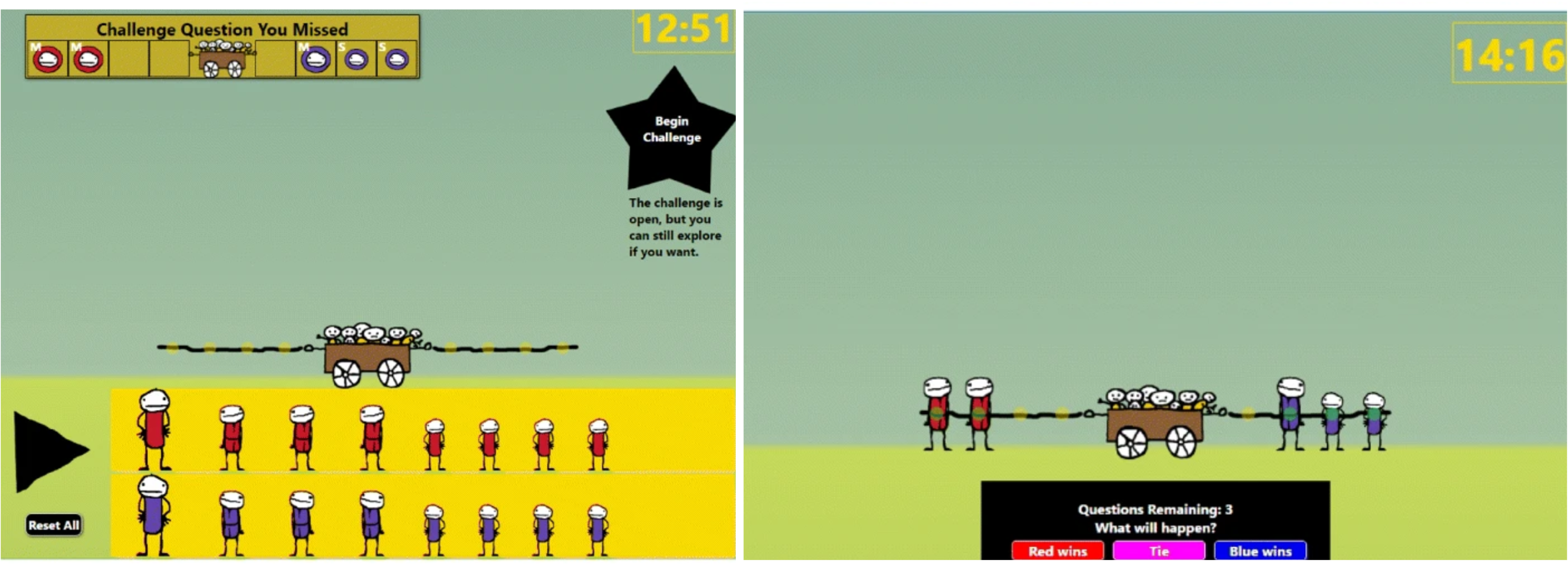
Environment. TugLet [7] is an open ended learning game designed to play in 2 modes: explore and challenge. Through the exploration, the students need to uncover the weights of 3 different characters through tug of war. In the challenge mode, they are tested on different tug-of-war configurations. If they answer wrong, students are redirected to the “explore" mode. Until then, they can freely switch between modes at their discretion. The game ends when a player successfully predicts the outcomes of eight consecutive configurations (See Appendix A.2).
For this study, a post-test consisting of 10 questions evaluated the extent to which players had acquired an understanding of the relationships among the various figure strengths.
Data Collection. The dataset employed in our research was
obtained through a classroom-based experiment conducted in
multiple middle schools encompassing a total of \(1746\) participating
students. We had partial information about teacher-reported sex
(\(146\) females, \(148\) males, \(1452\) were not reported) and country (country\(_-\) : \(468\)
and COUNTRY\(^+\) : \(1278\)). We note that country\(_-\) ranks 30+ places higher
than the COUNTRY\(^+\) on the Economic Complexity Index [1]. The
study was approved by the institutional ethics review board
(HREC 060-2020/04.09.2020)
Using the logs, we record each challenge or explore trial as: 1) the type of figures (large, medium, small or none) on each sides of the cart ; 2) whether the configuration ended in a tie or not (one-hot encoded, in challenge mode only), 3) whether the interaction was in explore mode, 4) whether the answer was correct (challenge mode only).
Label Mapping. We defined the high understanding students as
those who received a score of \(9\) or higher on the post-test. Indeed,
to achieve such a high score, students needed to understand all
the relations between the characters. Consequently, the
intervention (interv.) students were those who received a
score strictly lower than \(9\).
2.3 Student Success Prediction
2.3.1 Student Model Pipeline
For both OELEs, we used a simple network (GRU-Att) comprising of a Gated Recurrent Unit Cell followed by an Attention layer and a classification layer (Fig 1, top). We selected this architecture as it resembled the ones used in prior works on both datasets [6, 5]. We trained both classifiers to predict intervention needs for each student.
2.3.2 Ground Truth
We use the labels high (0 / true negatives) and intervention
(interv.) (1 / true positives) for each student as ground truth to train our predictors. Students are assigned to the group
interv. or high based on their performances on their
respective open ended learning environments, as described
to the paragraphs Label Mapping in Sections 2.2.1 and
2.2.2.
2.3.3 Model Evaluation
Due to the small size of both datasets, we used 10000
runs of bootstrap sampling with replacement on the test
set predictions to compute our classification scores (areas
under the ROC curve, false positive rates, false negative
rates and F1 scores) [16]. Indeed, computing the scores as
the average over folds would mean to compute the score
on less than \(10\) instances per fold for the minority group.
Specifically, we computed classification performances over the
whole population \(\mathcal {U}\), the chosen minority group \(\mathcal {U}^m\) and its
complementary majority group \(\mathcal {U}^M\) at each run. We reported the
mean and \(95\%\) confidence interval for each metric and each
subpopulation over the 10000 bootstrapping runs. To compute
the False Positive Rates (FPR) and False Negative Rates
(FNR), we used the Youden statistical test to choose the
optimal threshold to turn the raw predictions into high
or intervention predictions [23, 15]. We used both of
these metrics to compute the F1 score and assess equalized
odds [12].
2.4 Tools to Investigate Biases Across Demographics and Levels of Understanding
To analyze the behavioral patterns between different demographic subpopulations and the relationships of these patterns to student success, we used Differential Sequence Mining and Fischerian Random Invariance tests to analyse the input sequences and outputs of the GRU and Attention layers of the models.
2.4.1 Pattern Mining
We employed two different pattern mining algorithms, the first one focusing on the sequential nature of the behavioral interactions and a second one focusing on analysing the outputs of the GRU and Attention layers of the network.
Differential Sequential Mining (DSM). We implemented the DSM algorithm as described in [8] and implemented by [14] to perform asymmetric comparisons. DSM is a three-step comparative algorithm. We start by defining 2 non overlapping groups to compare: \(\mathcal {U}^{\texttt {m}_-}\) and \(\mathcal {U}^{\texttt {M}^+}\). Step 1 is applied separately in each of these groups and consists in computing the student support (s-support). For each possible pattern, we count the proportion of students expressing that pattern. We call the patterns with a s-support\(\geq 0.5\) frequently expressed by the population. Step 2 consists in computing the interaction support for each pattern and each student, that is to compute how many times that pattern appears in each student’s interaction. Step 3 compares the distribution of i-supports of a pattern across the 2 non overlapping groups of students with a fisherian random invariance test to see if that pattern is significantly (\(p\leq 0.05\)) more expressed in the group with the highest average i-support. In doing so, we end up with 3 types of patterns: 1) the common interaction patterns: the patterns which are commonly expressed in both \(\mathcal {U}^{\texttt {m}_-}\) and \(\mathcal {U}^{\texttt {M}^+}\), 2)/3) the patterns specific to group \(\mathcal {U}^{\texttt {m}_-}\)/\(\mathcal {U}^{\texttt {M}^+}\): patterns that significantly appear more in a group regardless of whether they are also present in a majority of students in group \(\mathcal {U}^{\texttt {M}^+}\)/\(\mathcal {U}^{\texttt {m}_-}\).
Fischerian Random Invariance Test To investigate the behavior of the student models, we compared the values of the GRU and Attention layers output for different subgroups. To that effect, we applied a Fischerian Random Invariance test to each of the output values of the output vector individually, across 2 pre-defined subgroups of our users. We ended up with 2 types of output patterns: 1) the specific output patterns: output patterns which significantly vary across subpopulations, 2) the common output patterns: output patterns which do not significantly vary across different subpopulations. (See Appendix B)
2.4.2 Comparison Protocol
Demographic attributes Finally, we denote LANGUAGE\(^+\) the
language region with the most students \(\mathcal {U}_b\) and language\(_-\) the
language region with the least students in Beer’s Law. Similarly,
we call COUNTRY\(^+\) the country represented by the most students in
\(\mathcal {U}_t\) and country\(_-\) the country with the least amount of students in
TugLet. We recall the majority country has a lower socio-economic
status than that of the minority country. We focus on these
demographic attributes related to area for consistency
across datasets. We analyzed sex and gender on our github
repository3.
Comparison groups To understand whether different
demographics exhibited different inquiry behavior, we applied
each pattern mining to our features or output values to make 4
comparisons: comparison 1: \(\mathcal {U}^{\texttt {m}_-}_{\texttt {high}}\) vs \(\mathcal {U}^{\texttt {m}_-}_\texttt {interv.}\): different understanding
groups from the minority population, comparison 2: \(\mathcal {U}^{\texttt {M}^+}_{\texttt {high}}\) vs \(\mathcal {U}^{\texttt {M}^+}_{\texttt {interv}}\):
different understanding groups from the majority population,
comparison 3: \(\mathcal {U}^{\texttt {m}_-}_{\texttt {high}}\) vs \(\mathcal {U}^{\texttt {M}^+}_{\texttt {high}}\): different demographics groups from
the higher understanding level population, comparison
4: \(\mathcal {U}^{\texttt {m}_-}_{\texttt {interv}}\) vs \(\mathcal {U}^{\texttt {M}^+}_{\texttt {interv}}\): different demographics groups from the interv.
population. The first two comparisons were used as sanity
checks to evaluate the potential discriminative potential
(signal) between the high and interv. groups. The third
and fourth ones to establish any differences there may be
between two demographic groups of a same understanding
level.
3. RESULTS
3.1 RQ1: Student Models Performances and Biases
We trained and evaluated the models as described in Section
2.3.3. We ran a 10-fold cross validation on this grid: GRU cells
(\(4\), \(8\), \(16\)), Attention hidden size (\(4\), \(8\), \(16\)), epochs (\(30\), \(50\)). Based on ROC,
GRU cell \(16\), Attention hidden size \(16\) and epochs \(50\) were the best
parameters. Using bootrastrapping (Section 2.3.3), we observed
that the model trained on the Beer’s Law dataset performed
similarly across both \(\mathcal {U}^{\texttt {language}_-}\) and \(\mathcal {U}^{\texttt {LANGUAGE}^+}\) based on the bootstrapped AUC,
FPRs, FNRs and F1 scores as all confidence intervals overlap
(Figure 4 (TOP)). Conversely, we noticed a significant large (\(>0.1\))
gap in the F1 score across demographic groups in favour
of \(\mathcal {U}^{\texttt {country}_-}\) with no overlap of the confidence intervals (Figure
4 (BOTTOM)). Notably, the difference in AUC across
subpopulations was almost non-existent. This was explained by
the FPR being fairer to the country\(_-\) students while the FNR
was fairer to the majority group. For both datasets, a
consequent demographic imbalance exists: (Table 1). We would
have expected both student models to put these demographic
minority groups at a disadvantage. Yet, Beer’s Law model
seemed fair while TugLet’s model was biased towards the
majority \(\mathcal {U}^{\texttt {COUNTRY}^+}\) group. In the next subsection, we investigated the
behavioral differences across demographics and the output
values they generated. This, to understand where and why one
of them resulted in an unbiased model while the other one did
not.
| n° | group A [demo], [level] | group B [demo], [level] | patterns in common | A- specific | B- specific | alg. |
| Input Sequences
| ||||||
| 1 |
|
| \(21\) | \(6\) | \(0\) | DSM |
| 2 |
|
| \(16\) | \(8\) | \(2\) | DSM |
| 3 |
|
| \(23\) | \(7\) | \(1\) | DSM |
| 4 |
|
| \(15\) | \(5\) | \(0\) | DSM |
| GRU layer
| ||||||
| 5 |
|
| \(16\) | \(0\) | \(0\) | FRI |
| 6 |
|
| \(16\) | \(0\) | \(0\) | FRI |
| 7 |
|
| \(16\) | \(0\) | \(0\) | FRI |
| 8 |
|
| \(15\) | \(1\) | \(1\) | FRI |
| Attention Layer
| ||||||
| 9 |
|
| \(16\) | \(0\) | \(0\) | FRI |
| 10 |
|
| \(16\) | \(0\) | \(0\) | FRI |
| 11 |
|
| \(16\) | \(0\) | \(0\) | FRI |
| 12 |
|
| \(15\) | \(5\) | \(5\) | FRI |
| Prediction Layer
| ||||||
| \(13\) | FN |
| \(15\) | \(4\) | \(15\) | DSM |
| \(14\) | FN |
| \(16\) | \(2\) | \(8\) | DSM |
| \(15\) | FP |
| \(21\) | \(1\) | \(1\) | DSM |
| \(16\) | FP |
| \(16\) | \(9\) | \(2\) | DSM |
3.2 RQ2: behavioral differences
To understand whether different demographics exhibit different inquiry behavior, we applied Differential Sequence Mining (DSM) to the four comparisons described in Section 2.4.1. We refer to these comparisons by their enumerated number throughout the rest of this section, and refer to row \(s\) by \(RS\).
We started by examining the students from the Beer’s Law
dataset (Table 2). Through comparisons 1 and 2 (R1 and R2),
we found that there were \(6\) and \(10\) specific interaction patterns
between the high and interv. understanding groups for
language\(_-\) and LANGUAGE\(^+\) respectively. This let us extrapolate
that a student model could perform well because we interpreted
the presence of multiple unique interaction patterns in
each group as indicating that there was likely sufficient
signal to differentiate between target groups. All interaction
patterns from the high understanding students involved
actions in (sub)optimal conditions while the few interaction
patterns from the interv. students were actions made
in a non observable state (see Section 2.2.1). Through
comparisons 3 and 4 (R3 and R4), we found that \(\mathcal {U}^{\texttt {language}_-}\) stood out
with \(13\) specific interaction patterns of its own from the LANGUAGE\(^+\)
population which only had \(1\) specific interaction pattern. This,
showing that there were demographic behavioral differences in
this dataset too. For example, the students \(u\in \mathcal {U}^{\texttt {language}_-}\) differentiated
themselves by changing parameters or taking breaks in a
coherent or optimal state. These differences suggested
that the student models would work better for \(\mathcal {U}^{\texttt {language}_-}\) while the
higher number of differences across understanding levels in \(\mathcal {U}^{\texttt {LANGUAGE}^+}\)
indicated the opposite. These contradicting conclusions meant
that both effects could potentially counterbalance each
other. We carried out the same analysis on the TugLet
dataset (Table 3). Once again, we saw through comparison 1
and 2 (R1 and R2) that there are a lot of differences (\(28\))
between the high and intervention understanding groups for
both \(\mathcal {U}^{\texttt {country}_-}\) and \(\mathcal {U}^{\texttt {COUNTRY}^+}\). This indicated again that potentially helpful
signal to differentiate the two target groups (high and
intervention) is present in the dataset. No matter the
demographic-understanding level, all interaction patterns
specific to a group were from the challenge mode (see Section
2.2.2). Only the high understanding students managed to
answer a tie question correctly and go on to the next “challenge"
questions. Furthermore, we found demographic behavioral
differences for students with a similar understanding, but
different demographic attributes. This time, the odds were
in favour of the minority \(\mathcal {U}^{\texttt {language}_-}\) subpopulation as we observed
through comparisons 3 and 4 (row 3 and 4) that only the \(\mathcal {U}^{\texttt {country}_-}\)
subpopulation stood out and differentiated itself from \(\mathcal {U}^{\texttt {COUNTRY}^+}\)
subpopulation with \(13\) specific interaction patterns, all levels of
understanding considered. We noted that for all datasets
and all subgroups, all patterns specific to a group were
present, to a lesser extent, in the complementary group
too.
In short, both datasets presented demographic behavioral differences across students with a similar level of understanding. Through DSM comparisons, we found that both \(\mathcal {U}^{\texttt {language}_-}\) and \(\mathcal {U}^{\texttt {LANGUAGE}^+}\) populations had their own specific interaction patterns in the Beer’s Law dataset, but only the minority \(\mathcal {U}^{\texttt {country}_-}\) population stood out in the TugLet dataset.
3.3 RQ3: Layer Propagations
To understand the behavioral differences uncovered by DSM, we dived into the analysis of the GRU and Attention layers and conducted the same four comparisons as listed in Section 2.4.1, this time applying the Fisherian Random Invariance test (results shown on the GRU layer, Attention layer, and Prediction layer sections of tables 2 and 3).
We started with the Beer’s Law dataset (Table 2) and
conducted comparisons 1, 2 and 3 as sanity checks on both the
GRU (rows 5, 6, 7) and Attention layers (rows 9, 10, 11).
At first, it seemed that the discriminating power of the
algorithm must have laid on the linear layer as none of the
potential output patterns were specific to any particular
groups. However, when conducting comparison 4 (rows 8
and 12), we found that the differences across the interv.
students from different demographic groups were exacerbated
through the network. Delving further into our analysis,
we found that the false negative instances (FN) were the
most different to the high understanding students from
the minority group (row 13 Table 2) with \(19\) traits specific
to either one of the groups. The false positive instances
(FP), on the other hand, were the most different to the
interv. students from the majority group (row 16). This
indicated that the algorithm may tend to focus on the
majority group when identifying the high understanding
group. This in line with the findings from research question
2 (Section 3.2) where we found that \(\mathcal {U}^{\texttt {LANGUAGE}^+}_{\texttt {high}}\) had more specific
interaction patterns (\(7\)) than the \(\mathcal {U}^{\texttt {language}_-}_{\texttt {high}}\) (\(1\)) (rows 1, 2). It also
indicated that the algorithm focused on the minority group to
identify interv. students. As before, this followed the \(\mathcal {U}^{\texttt {language}_-}\)
population standing out from the \(\mathcal {U}^{\texttt {LANGUAGE}^+}\) population as seen from the
comparison on the input sequences through DSM (rows 3,
4).
The behavioral differences propagated more subtly through the
TugLet student model. As the network processed the features, it
improved at differentiating \(\mathcal {U}^{\texttt {country}_-}_{\texttt {interv.}}\) from \(\mathcal {U}^{\texttt {country}_-}_{\texttt {high}}\) (rows 5, 9), but regressed at
differentiating \(\mathcal {U}^{\texttt {COUNTRY}^+}_{\texttt {interv.}}\) from \(\mathcal {U}^{\texttt {COUNTRY}^+}_{\texttt {high}}\) (Table 3, rows 6, 10): the number of
output values significantly different across understanding levels
went from \(5\) in the GRU layer down to \(0\) in the Attention layer.
Furthermore, we found that the student model improved at
differentiating the majority \(\mathcal {U}^{\texttt {COUNTRY}^+}\) from the minority \(\mathcal {U}^{\texttt {country}_-}\). Indeed,
a majority (\(\geq 12\) out of \(16\)) of the output values for the GRU
and Attention layers were significantly different across
demographic groups of similar understanding levels. In other
words, it improved at differentiating demographic groups
throughout the network and regressed at differentiating
understanding levels for the majority group \(U^{\texttt {COUNTRY}^+}\). We continued with
the analysis of the output values of the last layer of our
GRU-Att: the raw predictions. From comparisons 1 and 2 on
the input sequences (Section 3.2), we noticed that the
interv. groups have more specific traits than the high
understanding groups. More specifically, the interv. group
from \(\mathcal {U}^{\texttt {country}_-}\) is the one with the most specific traits, as can also
be noticed through comparison 4. This may have led the
algorithm to over-focus on \(\mathcal {U}^{\texttt {country}_-}_{\texttt {interv.}}\) to determine whether someone
belonged to the interv. group. This is consistent with the
application of DSM to compare the false positive instances
(FP), comparison 7 and 8 in Table 3. Indeed, we find that the
FP are the closest to the users \(u\in \mathcal {U}^{\texttt {country}_-}_{\texttt {interv.}}\). In essence, they were almost
indistinguishable from one another as none of the output
values activated significantly differently (row 15). Similarly,
the instances from \(u\in \mathcal {U}^{\texttt {COUNTRY}^+}_{\texttt {interv.}}\) did not stand out from the FP even
though the FP instances had their own specific traits (row
16). Similarly, when doing the comparison with the false
negative instances (FN), we found that the students \(u\in \mathcal {U}^{\texttt {COUNTRY}^+}_{\texttt {high}}\) were the
closest to the FN (row 14) which was consistent with the
students \(u\in \mathcal {U}^{\texttt {country}_-}_{\texttt {high}}\) being the least distinctive group, leading the
algorithm to focus on its counterpart from the majority
population.
| n° | group A [demo], [level] | group B [demo], [level] | patterns in common | A- specific | B- specific | alg. |
| Input Sequences
| ||||||
| 1 |
|
| \(24\) | \(7\) | \(21\) | DSM |
| 2 |
|
| \(25\) | \(11\) | \(17\) | DSM |
| 3 |
|
| \(24\) | \(3\) | \(0\) | DSM |
| 4 |
|
| \(32\) | \(10\) | \(0\) | DSM |
| GRU layer
| ||||||
| 5 |
|
| \(9\) | \(7\) | \(7\) | FRI |
| 6 |
|
| \(11\) | \(5\) | \(5\) | FRI |
| 7 |
|
| \(4\) | \(12\) | \(12\) | FRI |
| 8 |
|
| \(2\) | \(14\) | \(14\) | FRI |
| Attention Layer
| ||||||
| 9 |
|
| \(5\) | \(11\) | \(11\) | FRI |
| 10 |
|
| \(16\) | \(0\) | \(0\) | FRI |
| 11 |
|
| \(1\) | \(15\) | \(15\) | FRI |
| 12 |
|
| \(1\) | \(15\) | \(15\) | FRI |
| Prediction Layer
| ||||||
| \(13\) | FN |
| \(24\) | \(0\) | \(5\) | DSM |
| \(14\) | FN |
| \(25\) | \(0\) | \(1\) | DSM |
| \(15\) | FP |
| \(35\) | \(0\) | \(0\) | DSM |
| \(16\) | FP |
| \(32\) | \(12\) | \(0\) | DSM |
In summary, our analysis revealed that Beer’s Law’s layers yielded consistent outputs across different levels of understanding, with a slight increase in signal observed among the demographic group with a interv. level. Additionally, we find that the TugLet model increased the signal to differentiate demographic groups and reduced that used to differentiate understanding levels from the majority \(\mathcal {U}^{\texttt {COUNTRY}^+}\).

language\(_-\) and LANGUAGE\(^+\) on the Beer’s Law dataset,
(BOTTOM) the entire population, country\(_-\) and COUNTRY\(^+\) on
the TugLet dataset
4. DISCUSSION AND CONCLUSION
Open Ended Learning Environments’ advantages are two-fold: they enable students to learn specific scientific concepts on top of training transversal skills such as inquiry learning. Using behavioral traces on such environments to predict early student success or struggle has become routine [21]. Unfortunately, some of these predictive models may be biased towards certain demographic groups. In this paper, our primary focus was to gain a better understanding of how demographics, behavioral interactions and representation proportions played a role in shallow student models’ fairness. We conducted our investigation using small datasets obtained from two different open-ended learning environments, namely, Beer’s Law and TugLet which were implemented in high- and middle-school settings respectively. Despite the considerable differences between these educational contexts, both datasets contained valuable information including students’ short-term behavioral sequences of interaction and demographic attributes. In both cases, the primary objective of the student models was to identify students at risk of academic challenges solely based on their behavioral interactions with the platform, thereby enabling timely intervention and support between their course activities and the final evaluation. Using both these environments, we answered the following research questions: 1) Are underrepresented groups at a disadvantage in student models?, 2) Can we verify that different demographics express different behaviors on OELEs?, 3) How do these differences affect fair predictions and propagate through student models?
For the first research question, we trained and assessed two GRU-Att models and observed whether the under represented demographic groups were treated unfairly by our algorithms. With Beer’s Law, we found that there were no treatment differences across language regions. On the contrary, for TugLet, we found performance discrepancies across the minority and majority countries, unexpectedly in favour of the minority group. To understand why that was, we applied Differential Sequence Mining (DSM) to the behavioral sequences of interactions and identified demographical differences in both datasets, answering research question 2. Specifically, we found that both \(\mathcal {U}^{\texttt {language}_-}\) and \(\mathcal {U}^{\texttt {LANGUAGE}^+}\) had distinctive interaction patterns that differentiated them from the other demographic group. However, in the case of TugLet, only the minority \(\mathcal {U}^{\texttt {country}_-}\) stood out with its own specific interaction patterns. If we assumed that the potential biases which could propagate through this paper’s pipeline are Data to Algorithm biases [12], it is coherent with the former Beer’s Law model not presenting any significant biases as both groups standing out meant they counter balanced each other; and coherent with the latter TugLet model favoring the minority group. Through our analyses, we found that this bias wouldn’t be a representational bias as described in [12], but a variation which we called signal bias: where one of the two groups has more distinctive traits than the other no matter if they represent the majority of the dataset. More formally, we defined signal as the presence or degree of discernible differences or patterns between the groups that we aim to classify. Consequently, a dataset with high signal contains substantial variations or distinct characteristics among the groups, making it easier to use these differences as input features for classification tasks. On the other hand, a dataset with low signal lacks clear or specific traits that differentiate the groups, posing challenges in accurately classifying them due to the absence of pronounced differences.
To verify the signal bias hypothesis, we investigated how the
found demographical differences propagated through the
network via Fischerian Random Invariance tests and answered
research question 3. We found that the only differentiating
signal in the Beer’s Law model was between the interv.
understanding students of different demographic groups (\(\mathcal {U}^{\texttt {LANGUAGE}^+}_{\texttt {interv.}}\) versus
\(\mathcal {U}^{\texttt {language}_-}_{\texttt {interv.}}\)), implying that either the final predictive signal must be found
in the classification layer, or that the differentiating signal is a
composition-signal of different subgroups. That is, that there
are no traits common to the majority of all \(u\in \mathcal {U}_{\texttt {interv.}}\) or \(u\in \mathcal {U}_{\texttt {high}}\), but rather that
there exists multiple possible strategies in either \(u\in \mathcal {U}_{\texttt {high}}\) or \(u\in \mathcal {U}_{\texttt {interv.}}\), none of
them being used by a majority of the students, all of them being
used by the algorithm to make its final prediction. This
explains the null number of output patterns separating \(u\in \mathcal {U}_{\texttt {interv.}}\)
from \(u\in \mathcal {U}_{\texttt {high}}\), and the better-than-random performances of the
student model. On the other hand, we found that the TugLet
model seemed to be better at separating students from
different demographic groups rather than from different
understanding levels: the target at hand. This is in line with
our hypothesis about signal biases: original behavioral
differences across demographics are easier to learn than
these of different understanding levels, as the signal is
stronger across demographic attributes than understanding
levels. Consequently, it focuses on these differences rather
than on what it was trained for. This was strengthened by
our analysis of the misclassified instances that showed
that the algorithm focused on the minority \(\mathcal {U}^{\texttt {country}_-}\) group when
classifying interv. understanding students, the majority
target group of our dataset. Again, using the minority
group to classify instances which majoritarily belong to
the other demographic group led to the biased treatment
of that other group. In short, we found that in neither
of our datasets was the demographical minority group
put at a disadvantage. Surprisingly, the TugLet model
even favoured the underrepresented country\(_-\) population.
Through our three research questions, we found that a signal
bias might be the origin of these unfairness. Indeed, the groups
which stood out the most from the other ones and had more
differentiating interaction patterns between their target groups
(here understanding levels) appear to be at an advantage over
the others, no matter whether they are the majority or minority
group. Thus, we uncovered signal biases which occur when the
overrepresentations of distinctive traits seems to lead models to
focus on these differences. They thus overfit on the signal which
prevents them from generalizing well to the rest of the data.
As representational biases might be mitigated through
demographical resampling methods [12, 11], we hypothesize
that its variation signal bias may be mitigated through
behavioral resampling, according to how close/far away an
instance is from the students carrying the most signal.
Through this study, we thus draw attention on the importance
of focusing on behavioral differences in addition to the
demographic differences. Focusing on the \(\mathcal {U}^{\texttt {country}_-}\) students as a whole
would not have changed the proportion of signal for that
particular population as they already make up \(73\%\) of the data. A
cleaner approach would be to cluster separately the higher
and interv. students within a same demographic group
in order to find idiosyncratic traits across understanding
levels rather than across demographic ones. We would then
optimize the way the clusters are rebalanced based on the
signal measured across understanding levels before the
model is trained. Without such a deep analysis, the risks of
adding noise and therefore letting the algorithm over focus
even more on the population with the largest signal will
increase.
Nonetheless, we temper our conclusions by the limited realm of our investigation. A deeper investigation through more OELEs, different tasks, different populations, multi-target classifiers, and higher imbalance ratios would be required to generalize these findings. Furthermore, small noise and differences have a much greater impact on the classification performances which means that these conclusions could but may not be generalized to very large datasets. For these reasons, whether signal biases can be present in much larger datasets is still an open question. Finally, though this study has its limitation, we emphasize that considering behavioral biases is as important as considering demographic biases to hopefully offer equal education opportunities to the students and teachers we work to help.
5. ACKNOWLEDGEMENTS
This project was substantially financed by the Swiss State Secretariat for Education, Research, and Innovation SERI. Many thanks to Tanya Nazaretski, Jibril Frej, Vinitra Swamy, Seyed Parsa Neshaei and Kate Shved for their valuable help.
APPENDIX
A. OELES
A.1 Beer’s Law
In this simulation, the students can turn on the laser, change the wavelength of the laser, change the nature of the solution in the task and its concentration, change the width of the flask, change the dependent variable. Concentration, width and wavelength sliders can be directly changed by a clik on the desired value, or can be dragged to observe the continuous change. The independent variables influencing the absorbance are the width, concentration, and the wavelength of a laser. Their relationship with the dependent variable are linear, linear and colour-related respectively. The task designed to guide students’ inquiry was to rank 4 different configurations in terms of absorbance (Figure 2, bottom). They cannot just input the numbers into the simulation, as they are outside the allowed range on the environment. Thus, to successfully complete this task, students needed to plug in the numbers of the 4 configurations into the formula they extracted during their exploration.
A.2 Tuglet
Tuglet is a choice-based assessment in the form of a game designed to assess students’ inquiry strategies, in which students need to uncover the strengths of 3 characters through tug-of-war tests. The core concept of the game revolves around a tug-of-war scenario featuring two teams, each composed of figures with varying strengths categorized as large: \(3\), medium: \(2\), and small: \(1\) (Figure 3). Learners are given the choice to play in two distinct modes: the “explore" mode enables them to simulate different team compositions of up to \(4\) figures on each side of the cart and observe the resulting outcomes of tug-of-war matchups. The “challenge" mode, on the other hand, presents them with the task of predicting the outcome of specific tug-of-war scenarios followed by feedback indicating the correctness of the answer. In the event of an incorrect prediction, players are redirected to the “explore" mode for further exploration. Importantly, players retain the freedom to switch between modes at their discretion. The game ends when a player successfully predicts the outcomes of eight consecutive tug-of-war configurations, each progressively more challenging.
A.3 Feature processing - Beer’s Law
Features are similarly processed as in [6]. In particular, each click is characterized by: 1) the duration the student pressed on their mouse button , 2) the nature of the action (width, concentration, wavelength of the laser, type of solution, “other", “break") and 3) the configuration status of the system based on its usefulness to sucessfully complete the ranking task (optimal, suboptimal, coherent, or not observable). Breaks (time intervals between the clicks) are not explicitly recorded by the PhET environment. Therefore, still following the methodology described in [6], we inserted the 40% longest breaks in the interaction sequences as the shortest ones might be the logistic consequences of setting up an experiment and moving the mouse, rather than reflecting [6]. In short, the features used per students were thus sequential where each \(i_n\in S_u\) summarized a click into one vector.
B. FISCHERIAN RANDOM INVARIANCE TEST
![Algorithm 1: Fischerian Random Variance test over G1 and
G2, for n bootstrap runs
Require: G1 ∩G2 = ∅
μ1 ← mean(G1)
μ2 ← mean(G2)
δ(μ)= |μ1− μ2|
n1 ← size(G1)
ng2←←Gsize∪(GG2)
c ← 0 1 2
for run ← 1 to n do
Ga ← {} randomly assign n1 values from G to Ga
for a← 1 to n1 do
ra ← random(size(g)− r1 +1)
Ga.insert(G[ra])
eGnd f=orG∖ G
μab← meana(Ga)
μb ← mean(Gb)
if |μa − μb|≥ c then
c← c+ 1
end if
end focr
p ← n return p](./tmp-make4ht1x.svg)
C. REFERENCES
- Economic complexity index. Retrieved from https://oec.world/en/rankings/eci/hs6/hs96?tab=ranking, 2021. Accessed on 16.02.2024.
- B. Albreiki, N. Zaki, and H. Alashwal. A systematic literature review of student’ performance prediction using machine learning techniques. Education Sciences, 11(9), 2021.
- S. J. Caldas and C. Bankston. Effect of school population socioeconomic status on individual academic achievement. The Journal of Educational Research, 90(5):269–277, 1997.
- J. Cock, M. Marras, C. Giang, and T. Käser. Early prediction of conceptual understanding in interactive simulations. ERIC, 2021.
- J. M. Cock, M. Bilal, R. Davis, M. Marras, and T. Kaser. Protected attributes tell us who, behavior tells us how: A comparison of demographic and behavioral oversampling for fair student success modeling. In LAK23: 13th International Learning Analytics and Knowledge Conference, pages 488–498, 2023.
- J. M. Cock, M. Marras, C. Giang, and T. Käser. Generalisable methods for early prediction in interactive simulations for education. In Proceedings of the 15th International Conference on Educational Data Mining, page 183, 2022.
- T. Käser, N. R. Hallinen, and D. L. Schwartz. Modeling exploration strategies to predict student performance within a learning environment and beyond. In Proc. LAK, pages 31–40. ACM, 2017.
- J. S. Kinnebrew, K. M. Loretz, and G. Biswas. A contextualized, differential sequence mining method to derive students’ learning behavior patterns. Journal of Educational Data Mining, 5(1):190–219, 2013.
- S. Kippin and P. Cairney. The covid-19 exams fiasco across the uk: four nations and two windows of opportunity. British Politics, 17(1):1–23, 2022.
- S. M. Kong, K. M. Carroll, D. J. Lundberg, P. Omura, and B. A. Lepe. Reducing gender bias in stem. MIT Science Policy Review, 1:55–63, 2020.
- G. Lemaître, F. Nogueira, and C. K. Aridas. Imbalanced-learn: A python toolbox to tackle the curse of imbalanced datasets in machine learning. Journal of Machine Learning Research, 18(17):1–5, 2017.
- N. Mehrabi, F. Morstatter, N. Saxena, K. Lerman, and A. Galstyan. A survey on bias and fairness in machine learning. ACM Computing Surveys (CSUR), 54(6):1–35, 2021.
- P. Mejia-Domenzain, M. Marras, C. Giang, and T. Käser. Identifying and comparing multi-dimensional student profiles across flipped classrooms. In Proc. AIED, pages 90–102. Springer, 2022.
- S. Mishra, A. Munshi, M. Rushdy, and G. Biswas. Lasat: learning activity sequence analysis tool. In Technology-enhanced & evidence-based education & learning (TEEL) workshop at the 9th international learning analytics and knowledge (LAK) conference, Tempe, Arizona, USA, 2019.
- F. Pedregosa, G. Varoquaux, A. Gramfort, V. Michel, B. Thirion, O. Grisel, M. Blondel, P. Prettenhofer, R. Weiss, V. Dubourg, J. Vanderplas, A. Passos, D. Cournapeau, M. Brucher, M. Perrot, and E. Duchesnay. Scikit-learn: Machine learning in Python. Journal of Machine Learning Research, 12:2825–2830, 2011.
- S. Pfohl, Y. Xu, A. Foryciarz, N. Ignatiadis, J. Genkins, and N. Shah. Net benefit, calibration, threshold selection, and training objectives for algorithmic fairness in healthcare. In Proceedings of the 2022 ACM Conference on Fairness, Accountability, and Transparency, pages 1039–1052, 2022.
- R. D. Robnett. Gender bias in stem fields: Variation in prevalence and links to stem self-concept. Psychology of women quarterly, 40(1):65–79, 2016.
- H. Smith. Algorithmic bias: should students pay the price? AI & society, 35(4):1077–1078, 2020.
- V. Swamy, B. Radmehr, N. Krco, M. Marras, and T. Käser. Evaluating the Explainers: Black-Box Explainable Machine Learning for Student Success Prediction in MOOCs. In Proc. EDM, page 98, 2022.
- E. Tomul and H. S. Savasci. Socioeconomic determinants of academic achievement. Educational Assessment, Evaluation and Accountability, 24(3):175–187, 2012.
- A. Wang, V. V. Ramaswamy, and O. Russakovsky. Towards intersectionality in machine learning: Including more identities, handling underrepresentation, and performing evaluation. arXiv preprint arXiv:2205.04610, 2022.
- C. E. Wieman, W. K. Adams, and K. K. Perkins. Phet: Simulations that enhance learning. Science, 322(5902):682–683, 2008.
- W. J. Youden. Index for rating diagnostic tests. Cancer, 3(1):32–35, 1950.
- J. Zhang, X. Shi, I. King, and D.-Y. Yeung. Dynamic key-value memory networks for knowledge tracing. In Proceedings of the 26th International Conference on World Wide Web, pages 765–774, 2017.
1https://phet.colorado.edu/
2As this study was conducted in a multi-lingual country, the language area is officially considered as a demographic attribute.
3 https://github.com/epfl-ml4ed/behavioral-bias-investigation