ABSTRACT
We presented two empirical studies to assess the efficacy of two Deep Reinforcement Learning (DRL) frameworks on two distinct Intelligent Tutoring Systems (ITSs) to exploring the impact of Worked Example (WE) and Problem Solving (PS) on student learning. The first study was conducted on a probability tutor where we applied a classic DRL to induce policies using the training data collected from the same tutor. The second one was conducted on a logic tutor by leveraging a Multi-Task DRL framework to induce a Unified-DRL (U-DRL) policy from two related training datasets collected from the probability and logic tutors. Overall our results found that in the first study, the DRL policy significantly out-performs the Expert policy but no significant difference was found between the two policies on the number of PS and WE received. For the second study, while no significant difference between U-DRL and the Expert policy across various learning performance, the U-DRL students received significantly more PS and less WE than the latter. In short, our findings shows that 1) the efficacy of DRL policies is not necessarily enhanced when trained with multiple task-related datasets compared to a single source dataset; 2) the effectiveness lies not in how much PS and WE exposure students receive, but rather in how and when they are delivered.
Keywords
1. INTRODUCTION
Worked examples (WE) and Problem-Solving (PS) have a lengthy tradition of utilization in educational contexts for instructional purposes [60, 35, 31, 58, 61, 69]. In PS, students are assigned tasks to complete, either independently or with assistance, whereas in WEs, students are provided with detailed solutions. Generally speaking, presenting a WE is more passive since it often does not require students to act much; while PS is more active since it is expected that students would produce the solution with or without the tutor’s assistance. There has been a growing interest in utilizing WEs and PSs in e-learning environments such as Intelligent Tutoring Systems (ITSs) [39, 61, 45, 51, 42, 48, 74, 73, 72, 75, 70]. ITSs are interactive e-learning environments for enhancing students’ learning through tailored instruction, scaffolded practice, and on-demand assistance, demonstrating significant effectiveness [29, 63]. While the majority of current ITSs primarily emphasize PS, previous research indicates that integrating WE with PS can be more effective than relying solely on PS [38, 37, 39, 59].
In an ITS, the tutor’s decisions can be viewed as a temporal sequence, each of which affects the student’s successive actions and performance. Pedagogical policies are the decision-making policies inside an ITS that decide what action to take next in the face of alternatives. The sequential decision-making nature of Reinforcement Learning (RL) and Deep RL (DRL), combined with its ability to learn from a reward function, makes it a perfect fit to induce pedagogical policies for ITSs and optimize the learning process for each student individually. Indeed, a number of researchers have studied RL [44, 53] and DRL for pedagogical policy induction [10, 52, 36, 47, 46, 44, 12, 56, 22, 23, 75, 76]. Despite DRL’s great success, there are still many challenges preventing DRL from being applied more broadly in ITSs. One major problem is limited training data. It takes original DRL hundreds of millions of interactions with the environment to learn a good policy and generalize to unseen states, while we seek to learn policies from datasets with fewer than 1500 student-tutor interaction logs. While most of the prior work has mainly focused on inducing effective pedagogical policy using historical interaction logs collected from an individual ITS, relative little prior work has investigated building robust and unified pedagogical policy induction models using historical interaction logs collected across different ITSs.
In this work, we conducted two empirical investigations to evaluate the effectiveness of two DRL frameworks within two separate ITSs. In both studies, our emphasis was on examining the pedagogical choices related to Worked Example (WE) and Problem Solving (PS). The first study was conducted on a probability tutor by leveraging the classic Double Deep Q-Network [62] with Long-Short Term Memory [20] on the training data collected from the same tutor from previous year to induce a DRL policy. We then proposed a Multi-Task DRL framework combining Dreamer[18] and bisimulation metrics [16] to induce a Unified-DRL (U-DRL) policy. Our U-DRL framework addresses the challenge of data inefficiency through the implementation of Multi-Task Learning (MTL). This technique enables the transfer of valuable yet relevant knowledge across various tasks to enhance the learning capabilities of the RL agent. MTL excels in effectively training tasks with limited data, leveraging multiple task-related datasets during the DRL training process. Although in specific environments, such as Atari games, MTL improves both data efficiency and performance of the DRL policy, there is little empirical evidence that the multiple data trained DRL policy is always helpful to students in real world. Our second study was conducted on a logic tutor by leveraging U-DRL trained on two related training data collected from both the probability and logic tutors.
We have two research questions (RQs):
- RQ 1. Would a DRL policy trained using multiple
task-related data bring better learning effects to
students than a DRL policy trained using single-task
data?
- RQ 2. When deciding on the pedagogical preference between WE and PS, is it more effective for pedagogical policies to lean towards WEs or PS?
Overall our results found that in the first study, the DRL policy significantly out-performs an expert-designed policy but no significant difference was found between the two policies on the number of PS and WE received. For the second study, while no significant difference between U-DRL and an expert-designed policy on various learning performance, the U-DRL students received significantly more PS and less WE than the latter. In summary, our findings indicate the following: 1) The efficacy of DRL policies is not necessarily enhanced when trained with multiple task-related datasets compared to training on a single source dataset; 2) the effectiveness lies not in how much PS and WE exposure students receive, but rather in how and when they are delivered.
2. RELATED WORK
2.1 Problem Solving vs Worked Example
A manifold of research has studied the establishment of an adaptive education system that presents appropriate educational content according to the learning status of each learner [61, 45, 42]. One of the most significant research areas revolves around the question of whether pedagogical policies should prioritize PS or WE for students. PS has been a conventional strategy in ITS. Following [31], PS activities are considered beneficial to learning because they engage learners in active cognitive processing. Also, it can promote the transfer of knowledge or skills that are applicable beyond the specific tasks encountered in the tutoring system. Based on these advantages, the PS-centric strategy is frequently prioritized in ITS. However, there also has been some prior research on the positive impact on WE on learning. [58] suggests the advantage of WE such as reducing cognitive load or support for novice learners. Also, in [61], four conditions of PS-only, WE-only, WE-PS pairs, and PS-WE pairs (WE is used after PS) were compared in electrical circuits troubleshooting tasks and showed that WE-PS and WE-only groups outperformed the other groups. In terms of improvement of learning efficiency by WEs, [69] showed that students with WEs completed more tasks during a fixed time. Although these studies give an insight that a combination of PS and WE would be helpful, the question of whether PS or WE should be weighted more heavily also needs to be researched. [26, 71] already analyzed the frequency of PS and WE decisions in pedagogical decisions using policies such as RL to improve student learning, but still, there is no common consensus about this issue.
2.2 Applying RL & DRL to ITSs:
In ITSs, the student-ITS interactions can be described as sequential decision-making problems under uncertainty, which can be formulated as problems of RL, a learning paradigm that depends on long-term rewards without knowing the “correct" decisions at the immediate time-steps [57]. An increasing number of prior research has explored the use of RL and Deep RL (DRL) to ITSs (e.g. [30, 36, 47]) and specifically, it has showed that they can be used to induce effective pedagogical policies for ITSs [36, 65]. For example, Shen et al. [52] utilized value iteration algorithm to induce a pedagogical policy with the goal of enhancing students’ learning performance. Empirical evaluation results suggested that the RL policy can improve certain learners’ performance as compared to a random policy. Wang et al. [65] applied a variety of DRL approaches to induce pedagogical policies that aim to improve students’ normalized learning gain in an educational game. The simulation evaluation revealed that the DRL policies were more effective than a linear model-based RL policy. Recently, Zhou et al. [71] applied offline Hierarchical Reinforcement Learning (HRL) to induce a pedagogical policy to improve students’ normalized learning gain. In a classroom study, the HRL policy was significantly more effective than the other two flat-RL baseline policies. Ausin et al. applied a Deep Q-Network(DQN) algorithm to induce tutorial decisions between WE and PS[2], which inspires our model in the first case study. Ju et al. identified critical decisions in DQN based policy using long and short term rewards [27]. Most recently, Condor et al. applied an advanced DQN algorithm in ITS for providing automatic instructional feedback in an open-ended question[13]. In summary, prior studies suggest that RL and DRL can induce effective pedagogical policies.
2.3 Multi-Task Learning
Multi-Task Learning (MTL) is a technique where multiple similar tasks are learned simultaneously, thereby enhancing the model’s ability to perform each task [7]. By sharing knowledge across tasks, MTL can improve overall capabilities compared to models trained on single tasks. Additionally, MTL is expected to impart generalized abilities across all learned tasks [68]. This approach is particularly useful in fields such as computer vision, natural language processing, and education [15, 33, 40]. In the realm of RL, MTL holds promise as well. RL agents typically require extensive interactions with their environment to gather sufficient data for optimal solutions, which can be challenging in real-world settings. MTL offers a solution by leveraging information transfer when data collection is limited [32].
However, a key challenge for MTL in RL is reconciling differences in Markov Decision Processes across tasks. If task environments vary significantly, it becomes difficult to learn generalizable skills[64] or filter irrelevant knowledge. To address this challenge, many approaches[66, 54] have been proposed but a common strategy involves learning shared latent representations, which serve as general knowledge for all tasks [6, 14]. Extracting useful generalized knowledge directly from domains can facilitate the discovery of optimal policies for task performance [6, 14]. In our work, we propose to construct an integrated model for two ITSs based on this shared latent representation learning.
3. METHOD
In conventional RL, an agent interacts with an environment \(\mathcal {E}\) over a series of decision-making steps, which can be framed as a Markov Decision Process (MDP). At each timestep \(t\), the agent observes the environment \(\mathcal {E}\) in state \(s_t\); it chooses an action \(a_t\) from a discrete set of possible actions; and \(\mathcal {E}\) provides a scalar reward \(r_t\) and evolves into the next state \(s_{t+1}\). The future rewards are discounted by the factor \(\gamma \in (0, 1]\). The return at time-step \(t\) is defined as \(R_t = \sum _{t'=t}^{T} \gamma ^{t'-t} r_{t'}\), where \(T\) is the last time-step in the episode. The agent’s goal is to maximize the expected discounted sum of future rewards, also known as the return, which is equivalent to finding the optimal action-value function \(Q^*(s,a)\) for all states. Formally, \(Q^*(s,a)\) is defined as the highest possible expected return starting from state \(s\), taking action \(a\), and following the optimal policy \(\pi ^*\) thereafter. It can be calculated as \(Q^*(s,a) = \max _\pi \mathop {\mathbb {E}} [R_t | s_t=s, a_t=a, \pi ^* ]\) and \(Q^*(s,a)\) must follow the Bellman Equation.
In the following, we will describe the two DRL frameworks used in our two studies. For both studies, we evaluate our DRL-induced policies using an offline Off-Policy evaluation metric named Per-Decision Importance Sampling (PDIS)[43].
3.1 Per-Decision Importance Sampling (PDIS)
A primary challenge in RL and DRL for ITSs is the absence of reliable offline evaluation metrics. Much prior work applied RL and DRL work took an offline RL approaches to induce effective pedagogical strategies. This is done by first collecting a training corpus and the success of offline RL is often heavily dependent on the quality of the training corpus. One common convention is to collect an exploratory corpus by training a group of students on an ITS that makes random yet reasonable decisions and then apply RL to induce pedagogical policies from that training corpus. Empirical study is then conducted from a new group of human subjects interacting with different versions of the system. The only difference among the system versions is the policy employed by the ITS. The students’ performance is then statistically compared. Due to cost limitations, typically, only the best RL-induced policy is deployed and compared against some baseline policies.
On the other hand, we often have a large number of RL algorithms (and associated hyperparameter settings), and it is unclear which will work best in our setting. In these high-stake situations, one needs confidence in the RL-induced policy before risking deployment. Therefore, we need to develop reliable yet robust evaluation metrics to evaluate these RL-induced policies without collecting new data before being tested in the real world. This type of evaluation is called off-policy evaluation (OPE) because the policy used to collect the training data, also referred to as the behavior policy, is different from the RL-induced policy, referred to as the target policy to be evaluated. Previous work has shown that a Per-Decision Importance Sampling (PDIS)[43] is unbiased with lower variance while estimating the expected reward than simple IS [24].
PDIS is a type of Importance Sampling method that approximates the expected reward of the induced policy \(\pi \) by computing a ratio of the probability of the target policy \(\pi _{t}(a|s)\) to behavior policy \(\pi _{b}(a|s)\), as shown in Equation 1, where \(t\) is a time step and \(T\) is the terminal time of one trajectory. We applied soft-max transformation, shown in Eqn 2, to estimate target policy \(\pi _{t}(a|s)\) because it achieves a great alignment between the theoretical and empirical evaluation results for ITS[24]. For our validation data, we computed an average of PDIS values of each students learning trajectory. For PDIS, the higher the value of a policy, the more effective it is expected to be.
\begin {equation} PDIS_{\pi _{t}} = \sum \limits _{t=1}^{T}\gamma ^{t-1} (\prod \limits _{i=1}^{t} \frac {\pi _t(a_i|s_i)}{\pi _b(a_i|s_i)}) r_t \end {equation}
\begin {equation} \pi _{t}(a|s) = \frac {e^{Q(s,a)}}{\sum _{a' \in A} e^{Q(s,a')}} \end {equation}
3.2 Single-task DRL policy induction
3.2.1 Double Deep Q Network
Our DRL framework builds on Double Deep Q Network (Double DQN), a refined version of DQN aimed at tackling Q-value overestimation. \begin {equation} y := r + \gamma \max _{a_{t+1}}Q(s_{t+1},a_{t+1};\theta ^-) \end {equation}
From Equation 3, DQN estimates the target value \(y\) as the maximum Q-value by applying the target network. \(\theta ^{-}\). This substantially overestimates the target value in several Atari games[62]. To address this, in Double DQN, the main network \(\theta \) selects the best action, while the target network \(\theta ^-\) estimates the Q-value of the selected action. The loss function \(\mathcal {L}\) minimizes the gap between estimated Q-values and target values.
\begin {equation} a_{t} = \operatorname {argmax}_{a_{t}} Q(s_{t},a_{t};\theta ) \end {equation}
\begin {equation} y := r_t + \gamma Q(s_{t+1},\operatorname {argmax}_{a_{t+1}} Q(s_{t+1},a_{t+1};\theta );\theta ^-) \end {equation} \begin {equation} \mathcal {L} = \mathbb {E}\bigr [(Q(s,a;\theta )-y)^2] \end {equation}
While DQN and Double DQN share a similar structure, we used Double DQN as our baseline model due to its enhanced stability by avoiding Q-value overestimation in the next state and its great performance across various Atari games.[62].
3.2.2 Long Short Term Memory
We combined naive Double DQN with both fully connected and Long Short Term Memory (LSTM)[20] layers inspired by prior work of [2]. It can tackle long-term dependency issues in sequential data using gates to manage forgetting, updating, and outputting information. This architecture resolves the vanishing gradient problem seen in simpler recurrent networks. As our training data is the students’ learning trajectory based on long time sequences, we used LSTM as the main neural network.
In our DRL framework, we define states, rewards, and actions as follows. For the state \(s\), we explore two input configurations at time \(t\): one utilizing the three most recent state observations \(s_t, s_{t-1}, s_{t-2} (k = 3)\), and the other is four observations \(s_t, s_{t-1}, s_{t-2}, s_{t-3} (k = 4)\). Following [2], employing a pedagogical policy trained by DRL+LSTM with \(k = 3\) outperforms the policies with smaller \(k\) in ITS. Motivated by this finding, we adopt these input configurations to investigate the impact of higher values of \(k\). These inputs are sequentially processed through the LSTM layers. Concerning the reward function, we used Normalized Learning Gain(NLG = \(\frac {posttest - pretest}{1- pretest}\)), which can normalize the gap between a student’s posttest and pretest scores. Also, to explore the effectiveness of the pedagogical policy, we construct a model to approximate the value for the actions: PS or WE in a given state. To summarize, our policy is to estimate the state-action value function utilizing Double DQN and LSTM, given the choice of PS or WE, in three or four consecutive states per learning step. The trained policy will choose the action that results in the larger state-action value between PS and WE, as shown below. \begin {equation} a_{t} = \operatorname {argmax}_{a_{t}} Q(s_{t},a_{t};\theta ), a_{t} \in [PS, WE] \end {equation} where \(s_{t}^{k=3} = [s_t, s_{t-1}, s_{t-2}]\) or \(s_{t}^{k=4} = [s_t, s_{t-1}, s_{t-2}, s_{t-3}]\).
3.2.3 Single-Task DRL Training data
Our training dataset comprises problem-solving trajectories from 635 students over multiple semesters, from Fall 2016 to Spring 2021. We used accumulated learning experiences for 10 problems per student in the training phase to develop adaptive policies. To estimate state-action values, we utilize tutor decisions (PS or WE) at each step alongside relevant state features. The dataset encompasses 142 state features derived from pedagogical criteria used in prior studies[26, 21, 50], covering aspects like workload, time, difficulty, performance, and hints requested. Regarding rewards per step, we employ inferred rewards generated through a deep neural network[5] to distribute delayed rewards, as immediate rewards are only available at the end of each trajectory. We divided datasets in 90% for training and 10% for evaluation by adhering the same in prior works[1, 25, 27, 50]
Data Collection All student historical data(including second study) were obtained anonymously through an exempt IRB-approved protocol, and we scored them using double-blinded grading rubrics. All data were de-identified and no demographic data or grades were collected. This research seeks to remove societal harms that come from lower engagement and retention of students who need more personalized interventions for introductory Computer Science Courses.
3.2.4 DRL Policy evaluation
Table 1 presents the results of the Double DQN + LSTM policy with two input settings. The question label only indicates the problem order. It illustrates that the impact of input settings can vary depending on the problem. But no significant patterns emerged regarding which problem features favor one input setting over the other. Consequently, we opted for deploying policies mixing both settings for our initial experiment. Thus, our final DRL policy comprised 10 policies, one for each problem, with the policy highlighted in bold in Table 1 deployed for each respective problem.
| Question label | PDIS(\(k = 3\)) | PDIS(\(k = 4\)) |
|---|---|---|
| ex132 | 0.3810 | 0.2093 |
| ex132a | 0.0546 | 0.0378 |
| ex152 | 11.9814 | 0.6722 |
| ex152a | 0.0979 | 0.1810 |
| ex152b | 6.9842 | 0.3826 |
| ex212 | -6.2527 | -6.1222 |
| ex242 | 29.7481 | 92.3439 |
| ex252 | 9.7131 | 1.1763 |
| ex252a | 0.7554 | 0.0561 |
| exc137 | 0.1765 | 0.1599 |
3.3 Unified DRL policy induction
For the second experiment in logic tutor, we aimed to generate a Unified-DRL (U-DRL) policy, which is expected to be more effective than a single-task DRL policy by merging two different ITSs. As it is essential to find the general knowledge between two systems, we put two environments in latent space based on Dreamer[18] and merge them by applying bisimulation metrics[16].
3.3.1 Latent representation learning
Our methodology for inducing U-DRL policy is based on Dreamer, a model-based DRL in latent space environment[18]. It learns the latent dynamics model based on the Recurrent State Space Model(RSSM)[19] to predict and estimate the action and value model in latent space. Similarly, our model architecture for learning latent presentation was constructed as follows. We numbered our latent space model(1), value model(2) and action model(3). \begin {equation} \textbf {1.1) Encoder} : \hat {o}_{t} \sim \textit {enc}(o_t) \end {equation} \begin {equation} \textbf {1.2) Decoder} : o_t \sim \textit {dec}(z_t) \end {equation} \begin {equation} \textbf {1.3) Deterministic state} : h_{t} = f(h_{t-1},s_{t-1},a_{t-1}) \end {equation} \begin {equation} \textbf {1.4) Stochastic state} : s_{t} \sim f(s_{t}|h_{t}) \end {equation} \begin {equation} \textbf {1.5) Reward} : r_t \sim \textit {R}(z_t) \end {equation} \begin {equation} \textbf {2) Value} : v_t \sim \textit {V}(z_t) \end {equation} \begin {equation} \textbf {3) Policy} : a_t \sim \pi (a_{t}|z_t) \end {equation}
To elaborate on the model, the encoder/decoder pair resembles a variational autoencoder[28], which learns a latent space from input data through a probabilistic distribution. At time \(t\) and with batches from one of the ITS datasets \(\mathcal {B}\), our encoder embeds raw observations into a latent space \(\hat {o}^{\mathcal {B}}_{t}\sim enc(o^{\mathcal {B}}t)\), while the decoder reconstructs the original raw observation, \(o^{\mathcal {B}}t \sim dec(z^{\mathcal {B}}t)\), where the latent state \(z_{t}\) is a concatenation of deterministic and stochastic latent states. Moreover, we employed two distinct encoder/decoder sets for merging two ITS systems. Specifically, we constructed \(enc_1\) and \(enc_2\) for embedding raw observations into latent states \(\hat {o}_{t}^{ITS1}\) and \(\hat {o}_{t}^{ITS2}\), respectively, and \(dec_1\) and \(dec_2\) for reconstructing latent states to original observation states. Equations 10 and 11 explains our dynamics model, based on the RSSM architecture, which necessitates both deterministic and stochastic states. Here, the deterministic latent state is generated by a Gated Recurrent Unit[11], which typically outperforms RNN or LSTM in handling sequential data, while the stochastic latent state is estimated by the posterior probability \(p(s_t|h_t,\hat {o}_t)\) following the consideration of new observations.
3.3.2 Shared latent representation learning
Our main purpose for second study is to find out the latent space of two different ITSs and the shared latent representation, which means a combination of two different environments(MDPs) in ITSs. We suppose that this integration will improve capabilities in all tasks simultaneously learned since we use various related tasks for learning. Here, we used bisimulation metrics which can quantitatively measure how the two states in MDPs are behaviorally similar[16] for generating a shared latent state.
Bisimulation illutstrates a relationship between two different states in MDPs. It can cluster two states if they are behaviorally equivalent. Specifically, if the two states \(s_i\) and \(s_j\) have the same reward function \(R\) and transition probability \(p\) to the next bisimilar state, we can define the two states are bisimilar. The relationship can be defined as follow[17]. \begin {align*} &\textbf {Condition 1.} \hspace {0.2cm}\forall a \in A, R(s_i,a) = R(s_j,a)\\ &\textbf {Condition 2.} \hspace {0.2cm}\forall a, \forall C, \sum _{s' \in C}p(s_i,a,s') = \sum _{s' \in C}p(s_j,a,s') \end {align*}
, where \(C\) is the set of all clusters of states that are bisimilarly equivalent.
The limitation of the bisimulation relationship is too strict to be satisfied. The two states are no longer considered bisimilar if there are slight differences in reward and transition function. Bisimulation metrics[16], a pseudometrics-based distance that can measure how much the two states are behaviorally similar, can tackle this problem. The equation for bisimulation metrics is followed below. \begin {equation} Bisim(s_i,s_j) = \max _{a \in A} \bigr ( (1-c)|r_{s_i}^a - r_{s_j}^a| + cW_2(p_{s_i}^a, p_{s_j}^a)\bigr ) \end {equation} ,where \(c\) is a discount factor and \(W_2\) is a 2-Wasserstein distance between two different probability distribution. Here, the smaller the value, the more behaviorally similar the two states are. To make a generalized policy, we enforced the latent space model(equations 8 to 12) to contain the characteristics of bisimulation metrics. For that, by including a loss function in the latent space model, we approximated the L1 distance \(d\) between two latent states to be as same as bisimulation metrics as follows. We numbered our bisimulation metrics model as (4). \begin {equation} \textbf {4) Bisimulation metrics} : d(z_{t}^{i},z_{t}^{j}) \sim Bisim(z_{t}^{i},z_{t}^{j}) \end {equation} ,where \(z_{t}^{i} \in \mathcal {B}_{ITS1}\) and \(z_{t}^{j} \in \mathcal {B}_{ITS2}\) and each states is from batches by two ITS datasets, \(\mathcal {B}_{ITS1}\) and \(\mathcal {B}_{ITS2}\). This approach is inspired by [67] and [8]. [67] proposed a framework to find out domain invariant characteristics in different states using bisimulation metrics. By reducing irrelevant features, they provide a generalization ability and improved performance in a single task. [8] applies bisimulation metrics to transfer policy between two different MDPs.
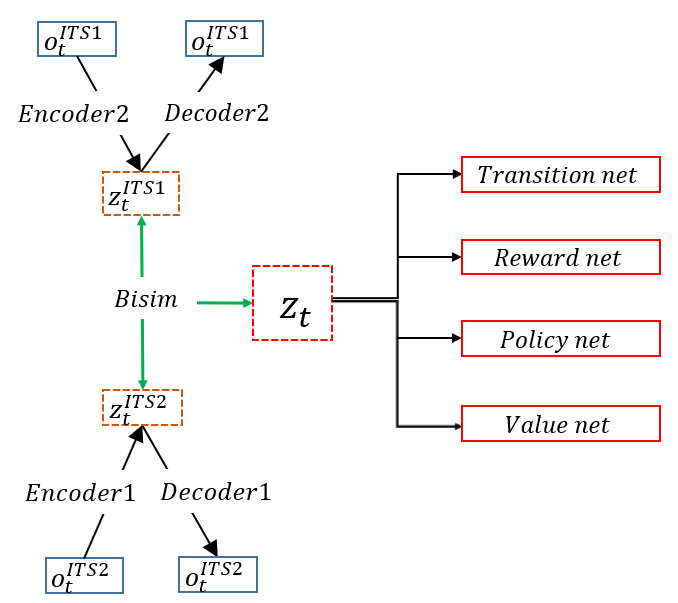
In summary, our U-DRL framework was initially constructed by following three parts: 1) latent space model(encoder, decoder, transition model, reward model), 2) bisimulation metrics in latent space, and 3)estimated value and action model. As lots of components are based on neural networks, we described the parameters in an Appendix A. The whole loss function during our model training can be defined as follows. \begin {equation} \mathcal {L} = \mathcal {L}_{latent} + \mathcal {L}_{value} + \mathcal {L}_{policy} \end {equation} \begin {equation} \mathcal {L}_{latent} = \mathcal {L}_{dec} + \mathcal {L}_{transition} + \mathcal {L}_{reward} + \mathcal {L}_{bisim} \end {equation}Our latent space model uses \(\mathcal {L}_{latent}\) as a loss function which is similar to that of Dreamer, where the \(\mathcal {L}_{dec} = -\mathbb {E}\bigr [\)ln \(p(o_t|z_t)\bigr ]\) and \(\mathcal {L}_{reward} = -\mathbb {E}\bigr [\)ln \(p(r_t|z_t)\bigr ]\) applying negative log-likelihood, transition loss (\(\mathcal {L}_{transition}\) = KL\((p(z_t|z_{t-1}\) \(,a_{t-1},o_t)||p(z_t|z_{t-1},a_{t-1})\)), value loss (\(\mathcal {L}_V = \frac {1}{2} ||v_{\psi }(z_t) - V_{\lambda }(z_t)||^2\)) where \(\psi \) is value network composed of FC layers and \(V_{\lambda }(z_t)\) is computed applying exponentially weighted average of rewards[18] , and policy loss (\(\mathcal {L}_\pi = - \mathbb {E} (\sum _{\textit {t}=t}^{t+H} V(z_\textit {t}))\)). Our framework combined them with the bisimulation loss (\(\mathcal {L}_{bisim} = ||z_{t}^{i} - z_{t}^{j}||_1-Bisim(z_{t}^{i}, z_{t}^{j}\))). Figure 1 shows how our U-DRL framework works. The training process can be summarized in three main steps. First, raw observations of each ITS domain are mapped into a latent state using different encoders. Second, the distance of latent states from each domain is trained to be the same as bisimulation metrics for generating shared latent states between each task. Third, the other properties like transition, reward, value, and policy networks are trained in the latent space.
3.3.3 U-DRL Training data
We used log data of both logic tutor and probability tutor for our training set. In logic tutor data, there are 1330 students’ trajectories of problem solving in the training phase from the Fall 17 to Fall 20 semester. We extracted 144 features following relevant prior work[49]. The reward function in logic tutor data is the difference between posttest and pretest scores divided by training time as the main purpose of logic tutor is maximizing learning performance while minimizing time for learning. In probability tutor data, there are 1148 students learning trajectories including 133 state features from Fall 16 to Fall 19 semester. The categories for feature selection are the same as that of logic tutor, but the inner elements are somewhat different because of the differences in the system and teaching subjects between the two ITSs. We applied normalization for each data and split 90% of students’ data into training data and the remainder for validation data. Here, we evaluate induced policy’s performance only for our experiment’s logic tutor task.
3.3.4 U-DRL Policy evaluation
| Model | PDIS |
|---|---|
| DQN+LSTM(\(k = 3\)) | 5991.92 |
| DQN+LSTM(\(k = 4\)) | 3958.61 |
| DDQN+LSTM(\(k = 3\)) | 5619.66 |
| DDQN+LSTM(\(k = 4\)) | 2007.60 |
| U-DRL | 6330.35 |
Table 2 displays the performance of U-DRL compared to other DRL policies. We computed the average of 50 PDIS values for the U-DRL policy because the latent state contains both deterministic and stochastic states, implying that the same raw observations can result in different latent states during evaluation. The results indicate that the PDIS value for the U-DRL policy surpasses that of the other four DRL models. Consequently, we conclude that the U-DRL policy theoretically outperforms single-task DRL models and have deployed the U-DRL policy to assess its effectiveness in a real-world environment.
4. TWO INTELLIGENT TUTORS
4.1 Probability tutor
Probability tutor is an ITS teaching fundamental probabilistic theory such as Bayes rule. It explicitly taught students how to employ a general principle to calculate the required probability of events. It can also provide immediate feedback for incorrect actions by students[9].
The learning process comprises four phases: Textbook, Pre-test, Training, and Post-test. In the Textbook phase, students receive an overview of the probabilistic theorem, helping them recall necessary principles. The Pre-test consists of 14 problems, without tutor feedback or hints.(This is the same in the post-test phase.) During Training, students tackle 12 problems sequentially, with the tutor’s intervention on problem type but not content. In the Post-test, students face 20 problems, including 14 problems isomorphic to the Pre-test and 6 non-isomorphic problems applying multiple principles. The students are graded similarly to the Pre-test.
Grading criteria The pre- and post-test problems required students to derive an answer by writing and solving one or more equations. We used three scoring rubrics: binary, partial credit, and one-point-per-principle. Under the binary rubric, a solution was worth 1 point if it was completely correct or 0 if not. Under the partial credit rubric, each problem score was defined by the proportion of correct principle applications evident in the solution. A student who correctly applied 4 of 5 possible principles would get a score of 0.8. The One-point-per-principle rubric in turn gave a point for each correct principle application. All of the tests were graded in a double-blind manner by a single experienced grader. The results presented below were based upon the partial-credit rubric but the same results hold for the other two. For comparison purposes, all test scores were normalized to the range of \([0,1]\).
4.2 Logic tutor
Logic tutor is an intelligent tutoring system teaching basic theories about propositional logic. It shows the premises and allows students to derive a required conclusion by applying logical axioms and theorems[55]. Many researchers have already applied effective techniques in logic tutor such as data-driven hints[41], problem selection[34, 41], or reinforcement learning[2].
Students progress through seven levels to complete the logic tutor’s learning process. The initial level features four questions, with the first two introducing the workflow and interface, followed by a pre-test of the next two questions solved independently. Levels 2 to 6 are training phase, where students tackle four out of eight problems per level. Three problems are tailored to the student’s performance level, while the fourth is a fixed and challenging level post-test problem. As logic tutor uses the same problem selection algorithm for all students, our pedagogical approach, utilizing DRL, focuses on selecting the problem type (PS or WE) for each student[3] in training phase. Finally, students take a post-test with more challenging problems than those encountered during training.
Grading criteria The scores for the pre-test and post-test are calculated by two criteria. One is the number of incorrect actions, and the other is the time for solving the problem. More specifically, a good score can be obtained by making small mistakes and taking less time to finish problem [3].
5. EXPERIMENT SETUP
For the probability tutor, the study was given to students as a homework assignment in an undergraduate Computer Science class in the Fall of 2022. Students were told to complete the study in two weeks, and they were graded based on demonstrated effort rather than learning performance. 79 students were randomly assigned into the two conditions: \(N=55\) for \(Expert\) and \(N=24\) for \(DRL\). It is important to note that the difference in size between the two conditions is due to the fact that we prioritized having a sufficient number of participants in the Control condition to compare the system performance across different semesters. During the training phase in the \(Expert\), a human-crafted Expert policy designed by an expert with over 15 years of experience was implemented to students. It alternates between reasonable instructional interventions while adhering to constraints. For instance, these constraints ensure students receive predetermined types of interventions at each level, as specified by instructors. The \(Expert\) policy is used as a baseline policy for comparing the effect of RL policy in a lot of previous works[2, 4, 25, 27]. Also, our induced policy was applied to train students who are in \(DRL\) condition. A t-test showed that there is no significant difference on average of pre-test score between \(Expert\) and \(DRL\) (\(t(77) = 1.487, p=0.146\)); with \(Expert\) and \(DRL\). This implies that no significant difference was found in the students’ incoming competencies between the two conditions.
For the logic tutor, the study was given to students as a homework assignment in an undergraduate Computer Science class in the Spring 2023 for two weeks. Students were randomly divided into the two conditions: \(N=37\) for \(Expert\) and \(N=29\) for \(U-DRL\). The way how policies are applied to students is same as the study on probability tutor. To assess the initial competence of students in \(Expert\) and \(U-DRL\) conditions, we followed the same way conducted on the first study. The results indicated no significant difference between \(Expert\) and \(U-DRL\) (\(t(64) = 0.003, p=0.907\)). This statistical analysis suggests that the initial competence levels of students in both conditions were similar.
6. RESULTS
6.1 DRL in probability tutor
| \(Expert\) | \(DRL\) | \(p\) value | |
|---|---|---|---|
| Pre-test | .796(.135) | .737(.171) | .146 |
| Iso-post | .812(.140) | .814(.228) | .126 |
| Iso-NLG | -.008(.619) | .351(.646) | <.05* |
| Post-test | .727(.144) | .765(.251) | <.05* |
| NLG | -.567(.772) | .140(.689) | <.05* |
| Training time | 87.43(30.79) | 88.47(31.05) | .892 |
| PSratio | 0.448(0.12) | 0.449(0.112) | .969 |
*The statistics with the prefix Iso only consider the 14 questions in the post-test that are isomorphic to the pre-test.
Table 3 summarizes the study results on the probability tutor, presenting average and standard deviations for seven performance measurements: Pre-test, Iso-post, Iso-NLG, Post-test, NLG, and PSratio. PSratio represents the ratio of PS decisions to total decisions in each student’s learning trajectory. To consider student competencies, NLG and Iso-NLG were analyzed. Initial analysis using ANCOVA test, with pre-test scores as covariates, focused on post-test scores and NLG for isomorphic problems. Results show no significant difference in Iso-post mean scores between \(Expert\) and \(DRL\) (\(F(1, 77) = 2.3992, p = .126\)), but significant differences in Iso-NLG (\(F(1, 77) = 4.652, p = 0.034, \eta ^2=0.06\)). In addition, ANCOVA tests revealed significant differences between \(Expert\) and \(DRL\) policies in Post-test (\(F(1, 77) = 8.296, p = 0.005, \eta ^2 = 0.1\)) and NLG (\(F(1, 77) = 11.9, p = 0.0009, \eta ^2 = 0.14\)). Overall, the \(DRL\) policy significantly outperforms the \(Expert\) policy in enhancing student learning.
For log analysis, we analyzed the training time in minutes at first and there is no significant differences between \(Expert\) and \(DRL\). Additionally, we analyzed the PS ratio in students’ learning trajectories to further understand the impact of PS but there is no statistically significant difference between the \(Expert\) and \(DRL\) condition. Based on the results, we can conclude that the way pedagogical decisions are presented to students has a greater impact on learning outcomes than simply adjusting the numerical ratio of PS to WE. In other words, how educational strategies are contextualized and delivered could play a more significant role in determining students’ learning gains compared to the specific balance between PS and WE tasks.
6.2 U-DRL in Logic tutor
| \(Expert\) | \(U-DRL\) | \(p\) value | |
|---|---|---|---|
| Pre-test | .512(.298) | .503(.258) | .907 |
| Post-test | .664(.208) | .608(.171) | .275 |
| NLG | .115(.482) | .003(.481) | .271 |
| Training time | 71.28(22.79) | 67.43(22.17) | .523 |
| PSratio | 0.49(0.08) | 0.65(1.06) | <.05* |
The study results for the logic tutor are presented in Table 4, mirroring Table 3. To account for the wide score range of the logic tutor, we analyzed learning performance using squared Normalized Learning Gains (\(\frac {posttest - pretest}{\sqrt {1- pretest}}\)), which reduces variance and differences between incoming competence groups. Following our result, we were unable to yield statistically significant evidence that our \(U-DRL\) outperformed the \(Expert\) policy. For post-test scores, an ANCOVA test with pre-test scores as covariates revealed no significant difference between \(Expert\) and \(U-DRL\) policies (\(F(1,64) = 1.381, p = 0.275\)). Similarly, the ANCOVA test for NLG scores showed no significant difference between the two policies (\(F(1,64) = 1.236, p = 0.271\)). Moreover, in terms of training time in minutes, a one-way ANOVA test using the condition as a factor found no significant difference in average training time between the two conditions (\(F(1,64) = 0.413, p = 0.523\)).
Although the NLG result is not statistically meaningful, our \(U-DRL\) policy is not capable of improving student performance compared with \(Expert\) policy. As the learning effect of the \(U-DRL\) policy was not significant, we decided to look at the impact of PSratio under both the \(Expert\) and \(U-DRL\) to identify the differences in terms of pedagogical decision. The PSratio of \(Expert\) is 0.49 and \(U-DRL\) is 0.66 and there were significant differences between the two groups (\(F(1,64) = 46.01\), \(p <.05\), \(\eta ^2=0.46\)). In other words, the students in \(Expert\) relatively take PS and WE in a balanced way, but the students in \(U-DRL\) tended to learn following PS-centered pedagogical decisions. Based on our NLG result, we can infer that the learning effect of the \(U-DRL\) policy, which made unbalanced decisions, may not be excellent.
7. CONCLUSIONS
In this study, we empirically examined the impact of PS and WE alongside DRL policies trained on various datasets across two ITSs. Initially, we utilized Double DQN and LSTM networks in the probability tutor domain, evaluating two input configurations to determine the most effective policy. Results revealed that the DRL policy significantly enhanced learning compared to an Expert policy, despite no significant differences in the distribution of PS and WE strategies. We then expanded our analysis to the logic tutor domain, aiming to capitalize on the benefits of Multi-Task Learning. However, the U-DRL policy, derived from shared latent representation learning, did not yield significant learning effects compared to an Expert policy and favored PS strategies. Hence, while DRL policies trained on diverse datasets may improve learning outcomes in certain domains, this effect is not consistent across all settings, and learning gains do not consistently align with PS-centric approaches or specific PS and WE proportions.
One potential reason on why our U-DRL fails to perform well is that we need more meaningful way to united the two training datasets. In this work, we leverage bisimulation metrics which assumes behavioral similarity encapsulating that states with similar observable behaviors are functionally equivalent. This assumption may not be valid with ITS and educational settings. Students can be provided a WE because he/she’s knowledge is too low and thus PS may cause frustration or when the student mastered all the knowledge and a WE would be more efficient than PS.
We believe this work provides a step forward in learning shared pedagogical policies across multiple ITSs. This method allows a single policy to learn from multiple datasets at the same time, to then optimize student learning across both tutors. However, we acknowledge the imperative for additional evaluation and testing. It is paramount that our method should undergo further scrutiny and validation across various tutoring systems to ascertain its robustness and effectiveness. Thus, our future work will focus on investigating the better offline off-policy evaluation (OPE) to develop a validity of induced DRL policy. Also, we will aim to refine the DRL policy based on MTL by collecting more stable and consistent data while simplifying the neural network structure to address issues related to data inconsistency and model instability.
8. ACKNOWLEDGMENTS
This material is based upon work supported by the National Science Foundation projects: Integrated Data-driven Technologies for Individualized Instruction in STEM Learning Environments (1726550), CAREER: Improving Adaptive Decision Making in Interactive Learning Environments (1651909). Any opinions, findings, and conclusions expressed in this material are those of the authors and do not necessarily reflect the views of the NSF.
9. REFERENCES
- M. Abdelshiheed, J. W. Hostetter, T. Barnes, and M. Chi. Leveraging deep reinforcement learning for metacognitive interventions across intelligent tutoring systems. In International Conference on Artificial Intelligence in Education, pages 291–303. Springer, 2023.
- M. S. Ausin. Leveraging deep reinforcement learning for pedagogical policy induction in an intelligent tutoring system. In In: Proceedings of the 12th International Conference on Educational Data Mining (EDM 2019),, 2019.
- M. S. Ausin. A Transfer Learning Framework for Human-Centric Deep Reinforcement Learning with Reward Engineering. North Carolina State University, 2021.
- M. S. Ausin, M. Abdelshiheed, T. Barnes, and M. Chi. A unified batch hierarchical reinforcement learning framework for pedagogical policy induction with deep bisimulation metrics. In International Conference on Artificial Intelligence in Education, pages 599–605. Springer, 2023.
- M. S. Ausin, M. Maniktala, T. Barnes, and M. Chi. Tackling the credit assignment problem in reinforcement learning-induced pedagogical policies with neural networks. In Artificial Intelligence in Education: 22nd International Conference, AIED 2021, Utrecht, The Netherlands, June 14–18, 2021, Proceedings, Part I, pages 356–368. Springer, 2021.
- D. Borsa, T. Graepel, and J. Shawe-Taylor. Learning shared representations in multi-task reinforcement learning. arXiv preprint arXiv:1603.02041, 2016.
- R. Caruana. Multitask learning. Springer, 1998.
- P. Castro and D. Precup. Using bisimulation for policy transfer in mdps. In Proceedings of the AAAI conference on artificial intelligence, volume 24, pages 1065–1070, 2010.
- M. Chi and K. VanLehn. Meta-cognitive strategy instruction in intelligent tutoring systems: how, when, and why. Journal of Educational Technology & Society, 13(1):25–39, 2010.
- M. Chi, K. VanLehn, D. Litman, and P. Jordan. Empirically evaluating the application of reinforcement learning to the induction of effective and adaptive pedagogical strategies. User Modeling and User-Adapted Interaction, 21:137–180, 2011.
- J. Chung, C. Gulcehre, K. Cho, and Y. Bengio. Empirical evaluation of gated recurrent neural networks on sequence modeling. arXiv preprint arXiv:1412.3555, 2014.
- B. Clement, P.-Y. Oudeyer, and M. Lopes. A comparison of automatic teaching strategies for heterogeneous student populations. In EDM 16-9th International Conference on Educational Data Mining, 2016.
- A. Condor and Z. Pardos. A deep reinforcement learning approach to automatic formative feedback. 2022.
- C. D’Eramo, D. Tateo, A. Bonarini, M. Restelli, J. Peters, et al. Sharing knowledge in multi-task deep reinforcement learning. In 8th International Conference on Learning Representations,\(\{\)ICLR\(\}\) 2020, Addis Ababa, Ethiopia, April 26-30, 2020, pages 1–11. OpenReview. net, 2020.
- T. Evgeniou and M. Pontil. Regularized multi–task learning. In Proceedings of the tenth ACM SIGKDD international conference on Knowledge discovery and data mining, pages 109–117, 2004.
- N. Ferns, P. Panangaden, and D. Precup. Bisimulation metrics for continuous markov decision processes. SIAM Journal on Computing, 40(6):1662–1714, 2011.
- R. Givan, T. Dean, and M. Greig. Equivalence notions and model minimization in markov decision processes. Artificial Intelligence, 147(1-2):163–223, 2003.
- D. Hafner, T. Lillicrap, J. Ba, and M. Norouzi. Dream to control: Learning behaviors by latent imagination. arXiv preprint arXiv:1912.01603, 2019.
- D. Hafner, T. Lillicrap, I. Fischer, R. Villegas, D. Ha, H. Lee, and J. Davidson. Learning latent dynamics for planning from pixels. In International conference on machine learning, pages 2555–2565. PMLR, 2019.
- S. Hochreiter and J. Schmidhuber. Long short-term memory. Neural computation, 9(8):1735–1780, 1997.
- J. W. Hostetter, M. Abdelshiheed, T. Barnes, and M. Chi. A self-organizing neuro-fuzzy q-network: Systematic design with offline hybrid learning. In Proceedings of the 2023 International Conference on Autonomous Agents and Multiagent Systems, pages 1248–1257, 2023.
- A. Iglesias, P. Martínez, R. Aler, and F. Fernández. Learning teaching strategies in an adaptive and intelligent educational system through reinforcement learning. Applied Intelligence, 31(1):89–106, 2009.
- A. Iglesias, P. Martínez, R. Aler, and F. Fernández. Reinforcement learning of pedagogical policies in adaptive and intelligent educational systems. Knowledge-Based Systems, 22(4):266–270, 2009.
- S. Ju, S. Shen, H. Azizsoltani, T. Barnes, and M. Chi. Importance sampling to identify empirically valid policies and their critical decisions. In EDM (Workshops), pages 69–78, 2019.
- S. Ju, X. Yang, T. Barnes, and M. Chi. Student-tutor mixed-initiative decision-making supported by deep reinforcement learning. In International Conference on Artificial Intelligence in Education, pages 440–452. Springer, 2022.
- S. Ju, G. Zhou, M. Abdelshiheed, T. Barnes, and M. Chi. Evaluating critical reinforcement learning framework in the field. In International conference on artificial intelligence in education, pages 215–227. Springer, 2021.
- S. Ju, G. Zhou, T. Barnes, and M. Chi. Pick the moment: Identifying critical pedagogical decisions using long-short term rewards. International Educational Data Mining Society, 2020.
- D. P. Kingma and M. Welling. Auto-encoding variational bayes. arXiv preprint arXiv:1312.6114, 2013.
- K. R. Koedinger, J. R. Anderson, W. H. Hadley, and M. A. Mark. Intelligent tutoring goes to school in the big city. 1997.
- K. R. Koedinger, E. Brunskill, R. S. Baker, E. A. McLaughlin, and J. Stamper. New potentials for data-driven intelligent tutoring system development and optimization. AI Magazine, 34(3):27–41, 2013.
- K. R. Koedinger, A. Corbett, et al. Cognitive tutors: Technology bringing learning sciences to the classroom. na, 2006.
- A. Lazaric and M. Ghavamzadeh. Bayesian multi-task reinforcement learning. In ICML-27th international conference on machine learning, pages 599–606. Omnipress, 2010.
- P. Liu, X. Qiu, and X. Huang. Recurrent neural network for text classification with multi-task learning. arXiv preprint arXiv:1605.05101, 2016.
- Z. Liu, B. Mostafavi, and T. Barnes. Combining worked examples and problem solving in a data-driven logic tutor. In Intelligent Tutoring Systems: 13th International Conference, ITS 2016, Zagreb, Croatia, June 7-10, 2016. Proceedings 13, pages 347–353. Springer, 2016.
- B. Liz, T. Dreyfus, J. Mason, P. Tsamir, A. Watson, and O. Zaslavsky. Exemplification in mathematics education. In Proceedings of the 30th Conference of the International Group for the Psychology of Mathematics Education, volume 1, pages 126–154. ERIC, 2006.
- T. Mandel, Y.-E. Liu, S. Levine, E. Brunskill, and Z. Popovic. Offline policy evaluation across representations with applications to educational games. In Proceedings of the 2014 international conference on Autonomous agents and multi-agent systems, pages 1077–1084. International Foundation for Autonomous Agents and Multiagent Systems, 2014.
- B. M. McLaren and S. Isotani. When is it best to learn with all worked examples? In International Conference on Artificial Intelligence in Education, pages 222–229. Springer, 2011.
- B. M. McLaren, S.-J. Lim, and K. R. Koedinger. When and how often should worked examples be given to students? new results and a summary of the current state of research. In CogSci, pages 2176–2181, 2008.
- B. M. McLaren, T. van Gog, C. Ganoe, D. Yaron, and M. Karabinos. Exploring the assistance dilemma: Comparing instructional support in examples and problems. In Intelligent Tutoring Systems, pages 354–361. Springer, 2014.
- I. Misra, A. Shrivastava, A. Gupta, and M. Hebert. Cross-stitch networks for multi-task learning. In Proceedings of the IEEE conference on computer vision and pattern recognition, pages 3994–4003, 2016.
- B. Mostafavi and T. Barnes. Evolution of an intelligent deductive logic tutor using data-driven elements. International Journal of Artificial Intelligence in Education, 27:5–36, 2017.
- A. S. Najar, A. Mitrovic, and B. M. McLaren. Adaptive support versus alternating worked examples and tutored problems: Which leads to better learning? In UMAP, pages 171–182. Springer, 2014.
- D. Precup. Eligibility traces for off-policy policy evaluation. Computer Science Department Faculty Publication Series, page 80, 2000.
- A. N. Rafferty, E. Brunskill, T. L. Griffiths, and P. Shafto. Faster teaching via pomdp planning. Cognitive science, 40(6):1290–1332, 2016.
- A. Renkl, R. K. Atkinson, U. H. Maier, and R. Staley. From example study to problem solving: Smooth transitions help learning. The Journal of Experimental Education, 70(4):293–315, 2002.
- J. Rowe, B. Mott, and J. Lester. Optimizing player experience in interactive narrative planning: a modular reinforcement learning approach. In Tenth Artificial Intelligence and Interactive Digital Entertainment Conference, 2014.
- J. P. Rowe and J. C. Lester. Improving student problem solving in narrative-centered learning environments: A modular reinforcement learning framework. In International Conference on Artificial Intelligence in Education, pages 419–428. Springer, 2015.
- R. J. Salden, V. Aleven, R. Schwonke, and A. Renkl. The expertise reversal effect and worked examples in tutored problem solving. Instructional Science, 38(3):289–307, 2010.
- M. Sanz Ausin, M. Maniktala, T. Barnes, and M. Chi. Exploring the impact of simple explanations and agency on batch deep reinforcement learning induced pedagogical policies. In Artificial Intelligence in Education: 21st International Conference, AIED 2020, Ifrane, Morocco, July 6–10, 2020, Proceedings, Part I 21, pages 472–485. Springer, 2020.
- M. Sanz Ausin, M. Maniktala, T. Barnes, and M. Chi. The impact of batch deep reinforcement learning on student performance: A simple act of explanation can go a long way. International Journal of Artificial Intelligence in Education, 33(4):1031–1056, 2023.
- R. Schwonke, A. Renkl, C. Krieg, J. Wittwer, V. Aleven, and R. Salden. The worked-example effect: Not an artefact of lousy control conditions. Computers in Human Behavior, 25(2):258–266, 2009.
- S. Shen and M. Chi. Reinforcement learning: the sooner the better, or the later the better? In Proceedings of the 2016 Conference on User Modeling Adaptation and Personalization, pages 37–44. ACM, 2016.
- A. Singla et al. Reinforcement learning for education: Opportunities and challenges. arXiv preprint arXiv:2107.08828, 2021.
- S. Sodhani, A. Zhang, and J. Pineau. Multi-task reinforcement learning with context-based representations. In International Conference on Machine Learning, pages 9767–9779. PMLR, 2021.
- J. Stamper, M. Eagle, T. Barnes, and M. Croy. Experimental evaluation of automatic hint generation for a logic tutor. International Journal of Artificial Intelligence in Education, 22(1-2):3–17, 2013.
- J. C. Stamper, M. Eagle, T. Barnes, and M. Croy. Experimental evaluation of automatic hint generation for a logic tutor. In International Conference on Artificial Intelligence in Education, pages 345–352. Springer, 2011.
- R. Sutton and A. Barto. Reinforcement Learning: An Introduction. MIT Press, 2018.
- J. Sweller. The worked example effect and human cognition. Learning and instruction, 2006.
- J. Sweller and G. A. Cooper. The use of worked examples as a substitute for problem solving in learning algebra. Cognition and Instruction, 2(1):59–89, 1985.
- F. J. Swetz. Capitalism and arithmetic: the new math of the 15th century, including the full text of the Treviso arithmetic of 1478, translated by David Eugene Smith. Open Court Publishing, 1987.
- T. Van Gog, L. Kester, and F. Paas. Effects of worked examples, example-problem, and problem-example pairs on novices’ learning. Contemporary Educational Psychology, 36(3):212–218, 2011.
- H. Van Hasselt, A. Guez, and D. Silver. Deep reinforcement learning with double q-learning. In Proceedings of the AAAI conference on artificial intelligence, volume 30, 2016.
- K. Vanlehn. The behavior of tutoring systems. IJAIED, 16(3):227–265, 2006.
- N. Vithayathil Varghese and Q. H. Mahmoud. A survey of multi-task deep reinforcement learning. Electronics, 9(9):1363, 2020.
- P. Wang, J. Rowe, W. Min, B. Mott, and J. Lester. Interactive narrative personalization with deep reinforcement learning. In Proceedings of the Twenty-Sixth International Joint Conference on Artificial Intelligence, 2017.
- A. Wilson, A. Fern, S. Ray, and P. Tadepalli. Multi-task reinforcement learning: a hierarchical bayesian approach. In Proceedings of the 24th international conference on Machine learning, pages 1015–1022, 2007.
- A. Zhang, R. McAllister, R. Calandra, Y. Gal, and S. Levine. Learning invariant representations for reinforcement learning without reconstruction. arXiv preprint arXiv:2006.10742, 2020.
- Y. Zhang and Q. Yang. A survey on multi-task learning. IEEE Transactions on Knowledge and Data Engineering, 34(12):5586–5609, 2021.
- R. Zhi, M. Chi, T. Barnes, and T. W. Price. Evaluating the effectiveness of parsons problems for block-based programming. In Proceedings of the 2019 ACM Conference on International Computing Education Research, pages 51–59, 2019.
- G. Zhou, H. Azizsoltani, M. S. Ausin, T. Barnes, and M. Chi. Hierarchical reinforcement learning for pedagogical policy induction. In International Conference on Artificial Intelligence in Education, 2019.
- G. Zhou, H. Azizsoltani, M. S. Ausin, T. Barnes, and M. Chi. Hierarchical reinforcement learning for pedagogical policy induction. In Artificial Intelligence in Education: 20th International Conference, AIED 2019, Chicago, IL, USA, June 25-29, 2019, Proceedings, Part I 20, pages 544–556. Springer, 2019.
- G. Zhou and M. Chi. The impact of decision agency & granularity on aptitude treatment interaction in tutoring. In Proceedings of the 39th annual conference of the cognitive science society, pages 3652–3657, 2017.
- G. Zhou, C. Lynch, T. W. Price, T. Barnes, and M. Chi. The impact of granularity on the effectiveness of students’ pedagogical decision. In Proceedings of the 38th annual conference of the cognitive science society, pages 2801–2806, 2016.
- G. Zhou, T. W. Price, C. Lynch, T. Barnes, and M. Chi. The impact of granularity on worked examples and problem solving. In Proceedings of the 37th annual conference of the cognitive science society, pages 2817–2822, 2015.
- G. Zhou, J. Wang, C. Lynch, and M. Chi. Towards closing the loop: Bridging machine-induced pedagogical policies to learning theories. In EDM, 2017.
- G. Zhou, X. Yang, H. Azizsoltani, T. Barnes, and M. Chi. Improving student-tutor interaction through data-driven explanation of hierarchical reinforcement induced pedagogical policies. In In proceedings of the 28th Conference on User Modeling, Adaptation and Personalization. ACM, 2020.
APPENDIX
A. PARAMETERS
A.1 Single Task DRL
Our neural net structure in DRL + LSTM consists of three LSTM layers with 1000 units, respectively, and one FC layer for the output. The FC layer has two units as the policy should compare two state action-value functions when PS and WE. All layers use a Rectified Linear Unit(ReLU) as the activation function. In addition, we use L2 regularization with penalty factor \(\lambda = 10^{-4}\) to prevent our model from being overfitting. We trained our model using 500 batches which are randomly selected from a static dataset for 150K steps.
A.2 Unified DRL
Our encoder comprises three FC layers with \(256\times 128 \times 64\) units. For the decoder, we used three FC layers with \(128\times 128 \times N\) units, where \(N\) is the number of features in raw observation. We used a recurrent state space model for the transition model, which consists of 32 latent units for each deterministic and stochastic state. The reward, policy and value net is also formed based on FC layers for estimating probability distribution given \(z_t\). For training, we sampled 64 batches with a length of 3 and used Adam as an optimizer. We have learning rates of \(6 \times 10^{-4}, 8 \times 10^{-5}, 8 \times 10^{-5}, 10^{-5}\) for latent space, value, action, and bisimulation model, respectively.
B. INTERFACE OF TUTORS
B.1 Probability Tutor
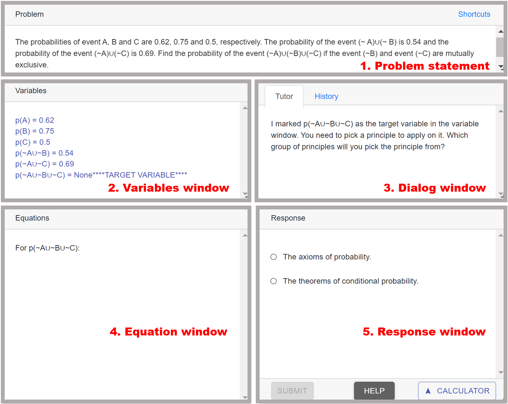
Figure 2 shows the interface of the probability tutor. The current problem is on the Problem statement window. The probabilities of events on the problems can be explicit or implicit(applying the problem in real life). In the Variables window, students can define variables by directly extracting them from problems or using probabilistic equations. Through the Dialog window, the tutor provides students feedback, hints, or instructions for the next step. From the Response window, students can interact with the tutors by selecting their next actions. Throughout the interaction, the equations required for solving the problem are displayed on the Equation window.
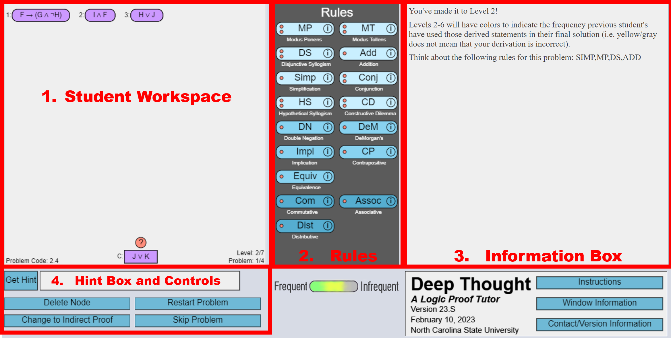
B.2 Logic Tutor
Figure 3 shows the first round of the PS step in logic tutor. If the current problem type is PS, students should solve the problem by themselves without any intervention from the tutor. As we can see, there are four main categories in the interface. First, in the student workspace, a procedure of student for deriving a goal statement is visualized. On the top of the workspace, three nodes of premises can be used for extracting conclusions. By applying propositional logic rules to the premises, students can finally reach the goal node at the bottom of the workspace. The question mark above the conclusion indicates that the problem is not solved yet. Second, there are fundamental logic theorems on the central window. Under the rules box is a frequency bar. This bar shows the frequency of how often the statements derived by students were used for concluding the past. Third, students can get a hint about which rules apply to the question in the information box. Lastly, on the hint and controls box, students can receive a direct hint for deriving rules by clicking the "Get Hint" box. Also, the other options in this part allow students to refresh, skip or solve the problem in indirect proof ways.