∗Work done during student internship at I2R, A*STAR
†Corresponding
author
ABSTRACT
Solving math word problems (MWPs) involves uncovering logical relationships among quantities in natural language descriptions of math problems. Recent studies have demonstrated that the contrastive learning framework can assist models in identifying semantically similar examples while distinguishing between different mathematical logics. This alleviates models’ dependence on shallow heuristics for predicting problem solutions. However, we have observed significant disparities in the positive and negative sample selections among different contrastive learning frameworks, which can sometimes exhibit complete contradictions. This discrepancy is attributed to the lack of an effective criterion for evaluating the distance between the mathematical logics of word problems. To address this issue, we introduce a novel formula for evaluating mathematical equation similarity in the context of word problem association. Our formula enables flexible focus on either global or local differences in the mathematical logic, thereby implementing distinct criteria for similarity calculation. We investigate the impact of various positive and negative sample selection strategies on contrastive learning models using the proposed formula in order to identify the optimal strategy. Our experimental results reveal substantial performance improvements over existing baselines, highlighting the effectiveness of our approach.
Keywords
1. INTRODUCTION
Math word problem (MWP) solving involves automatically
performing logical inference and generating mathematical
solutions from natural language-described math problems.
Recently, researchers have attempted to use different neural
networks for solving MWPs to avoid the tedious process of
manual feature construction.
While neural network-based models have significantly enhanced
performance on benchmark datasets, Patel et al. [16] argues
that state-of-the-art (SOTA) models rely on shallow heuristics
to solve the majority of word problems. These models frequently
face challenges even when addressing problems that exhibit only
minor textual variations.
| Problem 1 |
|---|
| Text: In Kaya’s teacher’s desk there are 9 pink highlighters, 8 yellow highlighters, and 5 blue highlighters. How many highlighters are there in all? |
| Equation: 9 + 8 + 5 |
| Prefix: + + 9 8 5 |
| Problem 2 |
| Text: In a sports club with 28 members, 17 play badminton and 19 play tennis and 2 do not play either. How many members play both badminton and tennis? |
| Equation: ( 17 + 19 + 2 ) - 28 |
| Prefix: - + + 17 19 2 28 |
| Problem 3 |
| Text: 70 students are required to paint a picture. 52 use green color and some children use red, 38 students use both the colors. How many students use red color? |
| Equation: 70 - 52 + 38 |
| Prefix: + - 70 52 38 |
Some studies utilize contrastive learning frameworks to assist models in discovering semantically similar examples while discerning those with different mathematical logics in a fine-grained manner [14, 12, 23]. The objective is to leverage similar logic to facilitate problem-solving and enhance the model’s sensitivity to subtle differences. One key aspect of contrastive learning is the construction of appropriate triplets. For each anchor data point \(P\) we find a logic-similar positive data point \(P^{+}\) and a negative data point \(P^{-}\) with different logic to form a triplet \((P,P^{+},P^{-})\). However, current contrastive learning frameworks struggle to formulate effective strategies for selecting positive and negative samples, to the extent that these strategies may exhibit complete contradictions with each other.
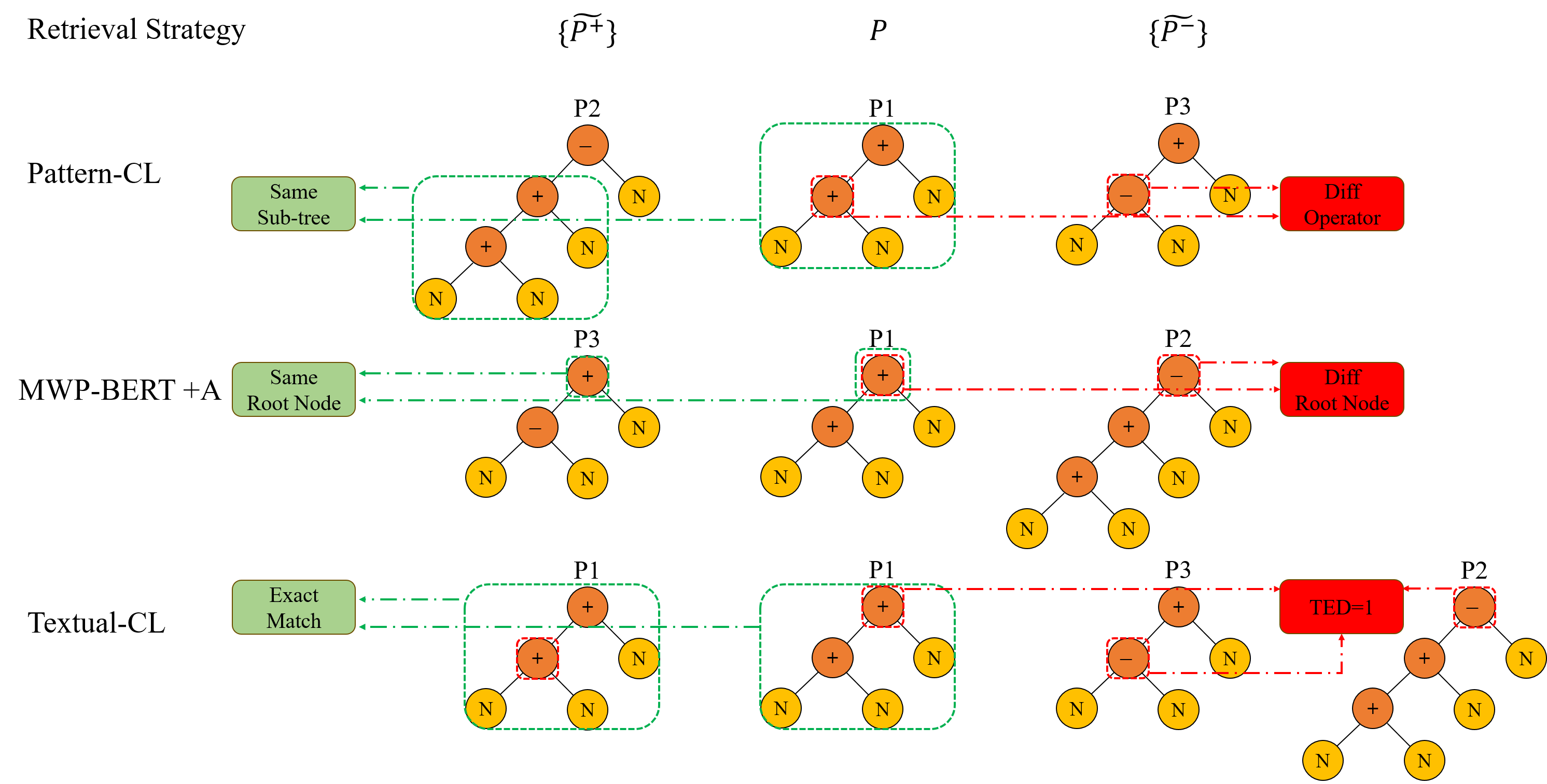
To demonstrate the contradiction in the positive and negative data points resulting from different selection strategies, we use a toy sample set consisting of only three MWPs, as presented in Table 1, as an illustrative example. For each problem, we construct a corresponding tree diagram representing its solution, as depicted in Figure 1. We then apply strategies from three representative contrastive learning frameworks for solving MWPs to highlight the contradictions in their results. Pattern-CL [12] utilizes positive and negative sample selection based on the sub-tree structure within the solution. Positive samples are chosen if they share the same abstract syntax sub-tree, while negative samples consist of those with the same abstract syntax tree but different operator nodes. MWP-BERT+Analogy [14] considers samples with the same root node in their abstract syntax trees as positive samples while the rest are regarded as negative samples. Textual-CL [23] considers samples with identical equations as positive samples. Negative samples are selected if their equations are similar but not identical, and the equation similarity is computed through Tree Edit Distance (TED) [17]. The positive and negative samples for MWP P1 are chosen within samples in Table 1 using the three selection strategies. The generated triplets are illustrated in Figure 1, where P2 is selected as positive and P3 as negative by Pattern-CL. The results are entirely opposite for MWP-BERT+Analogy. Textual-CL utilizes itself as positive and P2 or P3 as its negative with the TED of 1 if only the operator nodes are considered. As depicted, different and even contradictory triplets are constructed using only three samples. This issue would likely be more pronounced in a larger candidate pool.
The discrepancy arises due to the absence of a clearly defined distance or similarity measure between the logic structures of problems. It is challenging to intuitively discern which strategy is more appropriate. Pattern-CL and MWP-BERT+Analogy adopt a straightforward way to selection by directly comparing the same sub-tree and root node differences. They intentionally target different parts of the tree structure. On the other hand, Textual-CL utilizes Tree Edit Distance (TED) to quantitatively measure the similarity between two MWPs. However, TED assigns equal weight to operators at different levels of the tree, hindering its ability to differentiate between global and local structural differences. Another concern is that TED seeks to reduce dissimilarity between two trees by swapping left and right sub-trees of nodes that perform operations like subtraction, division, and exponentiation, where such swaps violate the inherent non-commutative properties of these operations.
Inspired by TED, we propose the Tree Level Weighted Distance (TLWD), a method for calculating equation similarity tailored specifically for MWPs. TLWD offers the flexibility to distinguish between root and leaf differences by adjusting the weights assigned to different levels of the equation tree. This enables us to generate various sets of positive and negative samples by focusing on either global or local logic structure. Thus, it facilitates the exploration of the impact of different triplet construction strategies on contrastive learning.
To summarize, the contributions of this paper are as follows:
- We demonstrate the inconsistency in the triplets construction strategies of current contrastive learning frameworks designed for MWPs.
- We propose a specific equation similarity calculation method for MWPs that empowers the baseline model with the flexibility to focus on local and global differences of problem logics.
- We conducted experiments using various positive and negative sample selection strategies derived from the proposed similarity measure, and provide guidance for the application of contrastive learning to address MWPs.
2. RELATED WORK
2.1 Math Word Problem Solving
Early studies usually address MWPs using either rule-based
methods or statistical methods to match problems to equation
templates [9, 18] with semantic parsing [19, 33]. Recently, a
deep learning-based approach inspired by sequence-to-sequence
(seq2seq) framework was proposed, emphasizing various designs
for both the encoder and decoder [28, 26, 27, 30, 13, 11].
Various neural networks, including recurrent neural networks
(RNNs)[28, 26, 27], graph neural networks [31], and the most
recent pre-trained models, such as BERT and its variants
[24, 13, 16], can be used as different encoders to extract and
aggregate information from the problem statements. More
recent studies have also focused on implementing more effective
decoders. For example, Xie et al. [30] introduced a goal-driven
tree structure decoder that enforces the model to predict math
equations following an exact tree structure. Treating the
solution as a Direct Acyclic Graph (DAG), Seq2DAG[2]
makes predictions in a bottom-up manner by aggregating
quantities and sub-expressions iteratively. A deductive
reasoning decoder [8] selects in each step two operands and
their operator in a bottom-to-top manner. The unified
tree decoder [1] alleviates the issue of multiple solutions
between input and output by predicting the solution in a
non-autoregressive way. Other studies leverage auxiliary tasks,
such as ranking and memory augmentation [21, 7], to improve
model performance.
Large language model (LLM) -based step-by-step math
reasoning [22, 25, 20, 5] is another recently explored research
direction, in which chains of thought or code explanations are
provided in addition to the final answer. However, the chains of
thought in natural language are not computationally executable,
and code explanations are computationally executable but
difficult for users who are not familiar with programming code
to interpret mathematically.
2.2 Contrastive Learning
Despite achieving relatively high performance on benchmark datasets, researchers have further challenged the understanding of the MWP solvers by introducing small variances [16] or employing adversarial attacks [10] on the problem text. The results demonstrate that current MWP solvers rely on shallow heuristics to solve the majority of word problems and struggle to detect subtle textual variances.
Contrastive learning was first introduced in computer vision
[3, 6] and subsequently adopted in MWP solvers aiming to
encourage models to pay attention to both the similarity and
subtle differences between problems [12, 14, 23]. Unlike
the perturbation-based augmentation [29] used in natural
language processing (NLP) to create positive samples for
contrastive learning, constructing positive and negative
samples in this manner cannot be directly applied to MWP
tasks. Researchers have attempted to seek similarity from
the logics of the problem solution to select positive and
negative samples [23, 12]. However, there is no fixed way to
determine the similarity or distinctiveness of the logics
between problems. As discussed in the introduction, different
or even contradictory positive and negative samples can
be selected for an anchor question by Pattern-CL [12],
MWP-BERT+Analogy [14] and Textual-CL [23]. An interesting
work by Zhang et al. [32] applied contrastive learning to
two different views of the solution from the top-down and
the bottom-up, avoiding the issue of selecting positive
samples.
3. THE PROPOSED APPROACH
For each anchor problem \(P=(T,E)\), where \(T\) represents the description of the problem and \(E\) represents the solution equation, a pair of positive data point \(P^{+}=(T^{+},E^{+})\) and negative data point \(P^{-}=(T^{-},E^{-})\) is constructed. This allows the use of contrastive learning to bring the representations of \(P\) and \(P^{+}\) closer to each other while pulling away the representations of \(P\) and \(P^{-}\). To determine the optimal way of selecting positive and negative samples for a given problem in a contrastive learning-based MWP solver, we propose Tree Level Weighted Distance, abbreviated as TLWD, to calculate the similarity between math equations and to represent the similarity of logics in problems with the flexibility to focus on differences either locally or globally.
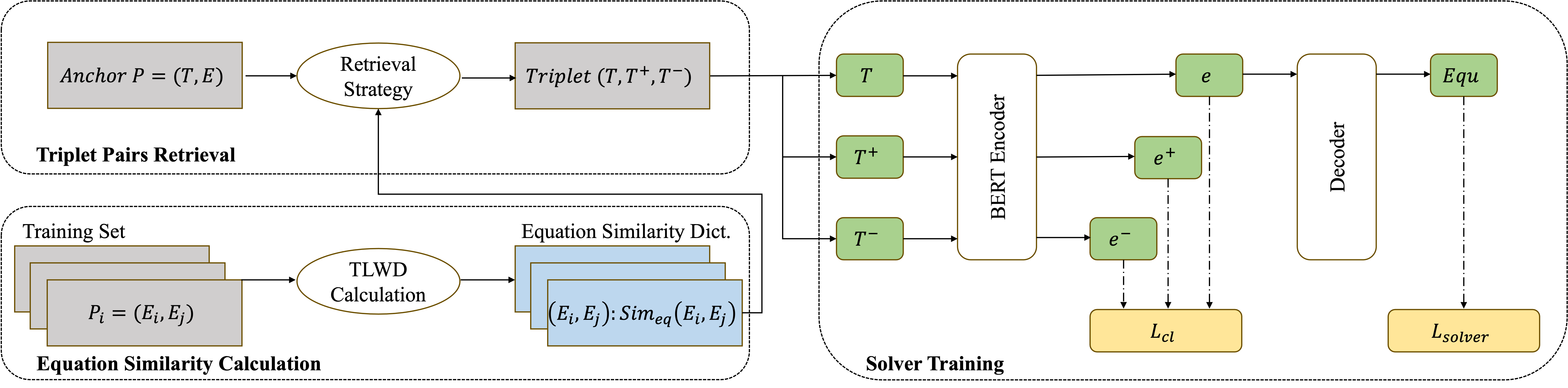
Following Shen et al. [23], we employ an equation similarity-based retrieval strategy, determined by the proposed TLWD, to extract positive candidate set \(\{{\widetilde P}^{+}\}\) and negative candidate set \(\{{\widetilde P}^{-}\}\). Our proposed training pipeline is illustrated in Figure 2. According to the pipeline, abstract syntax trees for all equations in training data are first constructed and normalized. Subsequently, we construct a dictionary \[(E_{i},E_{j}):Sim_{eq}(E_{i},E_{j})\] to record the similarities between the equation trees, which are then further used to construct the negative and positive candidate sets. Finally, we train the MWP solver, mapping T to E, by minimizing both the contrastive loss and the negative log likelihood loss for solution generation using the constructed training triplets derived from different retrieval strategies.
In the following subsections, we will explain the main components of the pipeline in detail.
3.1 Normalization
To normalize the equation trees, we consider operators and operands variables separately. We use variable unification (VU) on the numerical operands in the logic equation to avoid variations caused by different numerical values and apply the commutativity operation on the operators to normalize and simplify the logic equation.
3.1.1 Variable Unification
When selecting positive and negative samples, we unify the all the numerical variables in the solutions by replacing them with a common number placeholder \(N\), thereby disregarding differences between them. This step is crucial as it maps equations differing only in variable values to the same mathematical pattern, increasing the diversity of positive and negative samples for an anchor problem.
3.1.2 Commutativity Normalization
For a non-leaf node in a tree, commutativity normalization refers to an operation that swaps the left and right sub-trees of the current operator if it satisfies the following conditions: 1) the current operator is either addition or multiplication, 2) the length of the left sub-tree is less than that of the right sub-tree.
The commutative property holds for addition and multiplication operations, where the order of operands does not affect the final result. Based on this observation, we design commutativity normalization, through which we can transform two binary trees with seemingly significant structural differences into the same standardized binary tree.
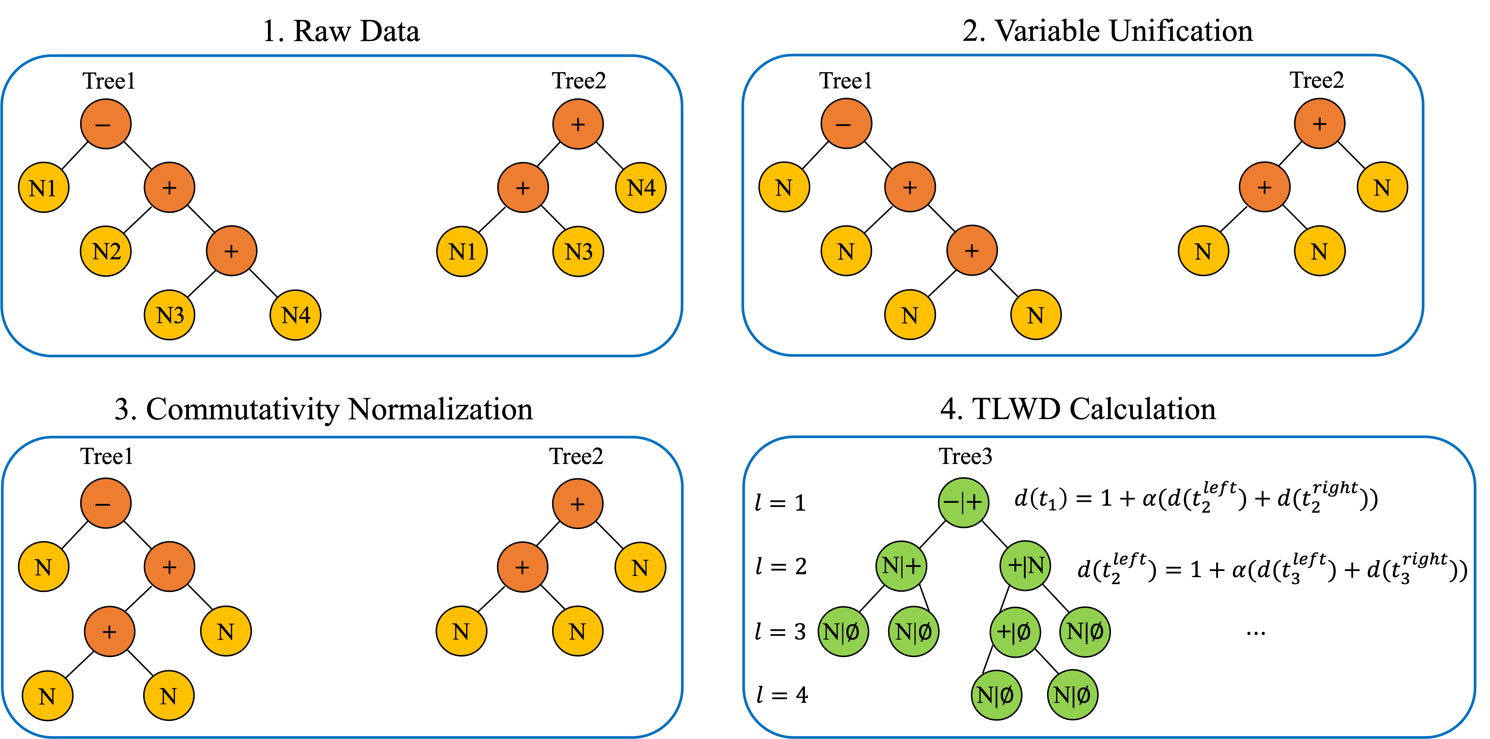
Commutativity normalization and TED differ in their approach to handling the swapping of left and right sub-trees in tree structures. While TED performs this swapping indiscriminately, regardless of the operator types involved. For example, TED may swap the sub-trees of the root node in Figure 3, potentially disrupting the logic of operations like subtraction. This can introduce logic violations. In contrast, commutativity normalization strictly perform swapping for commutative operators aiming to maintain the logical integrity of operations.
3.2 Tree Level Weighted Distance
Considering binary trees for two math problems, Tree1 and Tree2, our proposed TLWD recursively calculates the distance between the trees in three steps: overlapped tree construction, single node distance calculation, and recursive traversal over nodes from the bottom-up.
3.2.1 The Overlapped Tree Construction
To construct the common overlapped tree, denoted as Tree3, between Tree1 and Tree2, we focus on their structures and disregard the value of each node. The common overlapped tree refers to a tree that simultaneously encompasses the structures of both Tree1 and Tree2 in a minimal way. The process of common overlapped tree construction is illustrated in Figure 3, where the corresponding values of Tree1 and Tree2 at each node position are recorded in Tree3. If Tree1 or Tree2 lacks a certain node on Tree3, its value is recorded as Null.
3.2.2 Node Distance
The constructed overlapped tree records the differences between Tree1 and Tree2 at each node. By comparing value1 and value2 at each node of the overlapped tree, we can determine the distance between Tree1 and Tree2 at that node. The node distance of each node \(d(n)\) is defined as: \begin {equation} d(n)= \begin {cases} 0, & Value_{\text {1}} = Value_{\text {2}}\\ 1, & \text {otherwise}, \end {cases} \end {equation} where \(n\) denotes the node in one tree.
3.2.3 Tree Distance
A typical binary tree consists of a root node along with left and right sub-trees. Therefore, for a sub-tree with its root node at level \(l\), its tree distance \(d({t_{l}})\) can be defined as the sum of the node distance of its root node \(d({n_{l}})\) and the tree distance of its left and right sub-trees at level \(l+1\) in a recursive way: \begin {equation} d({t_{l}})=d({n_{l}}) + \alpha \cdot (d({t_{l+1}^{left}})+d({t_{l+1}^{right}})), \end {equation} where \(\alpha \) is the weighting coefficient on the left and right sub-trees, \(n_l\) denotes the node and \(t_l\) denotes the sub-tree at level \(l\). Varying the value of \(\alpha \) provides the flexibility to control the contribution of node distances at different levels to the total tree distance, enabling the model to focus on either local or global differences between the trees.
3.2.4 Interpretation of \(\alpha \)
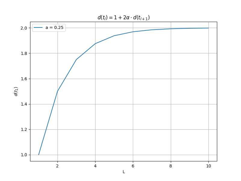
Let us delve deeper into the impact of the value of \(\alpha \) on the final TLWD. Assuming that none of the nodes in two abstract syntax trees are identical, we can observe from simulation, shown in Appendix A, that \begin {equation} d({t_{1}}) \to 2, \quad \text {when}\ \alpha = 0.25 \quad \text {and} \quad l \to \infty . \end {equation} The above suggests that when \(\alpha \) is set to 0.25, the root node’s distance carries more weight than the combined distance of all child nodes, indicating that differences near the root node have a greater impact on the TLWD of two abstract syntax trees. When \(\alpha \) is set to 1, \(TLWD\) considers the number of different nodes between the two abstract syntax trees to be the distance. This implies that nodes at different levels have equal distance weights, and the differences resulting from disparities in root nodes and leaf nodes are equivalent. When \(\alpha \) is greater than 1, the distance away from the root node increases exponentially as calculated recursively. In this scenario, distances far from the root node carry more weight, indicating that differences further from the root node have a more significant impact. By changing the value of \(\alpha \), we can determine the weight of differences in nodes at different levels when calculating the distance between two trees. This allows us to adjust retrieval strategies during positive and negative sample selection.
3.3 Equation Similarity
To retrieve the positive and negative samples, we evaluate the similarity between equations, i.e., \(Sim_{eq}\), based on the proposed \(TLWD\). The similarity of two equations \(E_{1}\) and \(E_{2}\) is then defined as: \begin {equation} \label {similarity_eq} Sim_{eq}(E_{1}, E_{2}) = 1 - \frac {TLWD(E_{1}, E_{2})}{TLWD_{max}(E_{1}, E_{2})}, \end {equation} where \(TLWD_{max}(E_{1}, E_{2})\) is the maximum tree distance of \(E_{1}\) and \(E_{2}\) where all node distances achieve their maximum, i.e., \(d(n) = 1\) for all nodes. Normalizing \(TLWD(E_{1}, E_{2})\) by the maximum tree distance \(TLWD_{max}\) restricts the values for the \(Sim_{eq}(E_{1}, E_{2})\) score to the range between \(0\) to \(1\).
3.4 WMP Solver and its Training
3.4.1 MWP Solver
We follow Li et al. [23] and use the baseline model BERT-GTS as our MWP solver. The pre-trained language model BERT [4], known for its robust textual representations, serves as the encoder in our approach. We utilize the goal-driven tree-structured (GTS) decoder [30] to systematically generate the prefix equation solution step by step, with a recursive neural network used to update sub-tree representations at each step. Given the target equation \(y=[y_1, y_2, ..., y_m]\), where \(m\) is the equation length, the solver generates \(k\)-th token \(y_k\) recursively, and the negative log likelihood is used as the generative loss computed as: \begin {equation} \mathcal {L}_{\mathrm {solver}} = \sum _{P} -\log \mathcal {P}(y|P), \end {equation} where \begin {equation} \mathcal {P}(y|P) = \prod _{k=1}^{m} \mathcal {P}(y_k|P) \end {equation} is the probability of \(y\) given \(P\).
3.4.2 Contrastive Learning
Contrastive learning operates on triplets \(z=(P,P^{+},P^{-})\), pulling closer the problem representations of \(P\) and \(P^{+}\) while pushing them away for \(P\) and \(P^{-}\). The contrastive loss used is given below: \begin {equation} \mathcal {L}_{cl}=\sum _{z} max(0,\eta +sim(e,e^{-})-sim(e,e^{+})), \end {equation} where \((e,e^{+},e^{-})\) is the encoder embedding of \((T,T^{+},T^{-})\), \(sim(\cdot )\) is the cosine similarity, and \(\eta \) is a margin hyper-parameter. The final training objective is to minimize \(L\), which is the sum of the generation negative log likelihood loss \(L_{solver}\) and the balancing parameter \(\beta \)-weighted contrastive learning loss \(L_{cl}\): \begin {equation} \mathcal {L}=\mathcal {L}_{solver}+\beta \cdot \mathcal {L}_{cl}. \end {equation}
3.4.3 Selection Strategy
We select the positive candidate set \(\{{\widetilde P}^{+}\}\) and the negative candidate set \(\{{\widetilde P}^{-}\}\) as follows:
- If there are examples with equations that are identical to that of the anchor, they form \(\{{\widetilde P}^{+}\}\).
- Otherwise, two strategies are considered: 1) \(\{{\widetilde P}^{+}\}=\{(T_{i},E_{i})\}\) satisfying \(argmax_{E_{i},T_{i}\neq T}(Sim_{eq}(E,E_{i}))\), containing samples with the nearest equation, which is known as the nearest neighbor (NN) selection strategy. 2) The anchor problem \(P\) selects itself as the positive sample. This, along with the aforementioned step for positive sample selection, is referred to as the exact match (EM) selection strategy.
- For the negative candidate set, we consider \(\{{\widetilde P}^{-}\}=\{(T_{i},E_{i})\}\) containing examples that satisfy \[argmax_{E_{i}\notin E\cup E^{+}}(Sim_{eq}(E,E_{i})),\] which holds the closest equation considering the positive example.
- We then randomly select one from each of the two sets and construct a triplet \((P, P^{+}, P^{-})\).
4. EXPERIMENTS
We conducted experiments on three widely-used real datasets to answer the following questions:
- How does our proposed strategy select the positive and negative samples for the anchor question compared to existing selection strategies? To which level of the math equation should we pay attention to in order to improve the model’s prediction accuracy?
- How good would the performance be for baseline models if they used our proposed strategy instead of the existing ones?
4.1 Datasets and Experimental Settings
The three datasets that we used for the experiments include: Math23k [23], a Chinese dataset consisting of 23,162 problems (21,162 for training, 1,000 for validation, and 1,000 for testing); MathQA [14], an English dataset at GRE level and ASDiv-A [15], a dataset of relative simple MWPs mostly with one to two operators. For MathQA, we follow the latest version used in [14], which includes the four arithmetic operators \(+,-,*,/\) with 16191 training samples and 1605 testing samples. We evaluated all three datasets using the accuracy metric, which checks whether the numerical answers of the model’s equation solutions matches the ground truth values.
The baseline models utilized in this paper can be categorized into those employing contrastive learning and those that do not. For solvers without contrastive learning, we selected GTS [30] and Graph2Tree [31] which are the most commonly-used baselines in other papers. For solvers with contrastive learning, we investigated three strong baseline contrastive learning models: Pattern-CL [12], Textual-CL [23] and MWP-BERT+Analogy[14].
Our model was trained and evaluated using Pytorch with a single NVIDIA RTX 4090 GPU. We used language-specific BERT model as the problem encoder. BERT base model is used for English datasets of MathQA and ASDiv-A and its Chinese version is used for Math23K. Following Shen et al. [23], the maximum input length of the BERT model was set to 256, and the maximum length of equation generation for the decoder was set to 45. The embedding size used for the decoder was 128. We trained the model on Math23K and MathQA for 120 epochs and on ASDiv-A for 50 epochs, using a batch size of 16 and a learning rate of 5e-5. The loss margin \(\eta \) was set to 0.2. The weight \(\beta \) for the contrastive learning loss was set to 5.
4.2 Comparative Experiments
| Model | Math23k | MathQA | ASDiv-A |
|---|---|---|---|
| Solvers w/o CL
| |||
| GTS | 75.6 | 68 | 68.5 |
| Graph2Tree | 77.4 | 69.5 | 71 |
| BERT-GTS | 82.4^* | 74.3 | 73.4 |
| Solvers w/ CL
| |||
| Pattern-CL | 83.2 | 73.8^* | - |
| Textual-CL | 84.1 | 74 | 74.2 |
| MWP-BERT+Analogy | 85.1 | - | - |
| BERT-GTS+TLWD(ours) | 85.5 | 75.4 | 75.9 |
| Variable Unification | Operator Normalization | Acc.
| ||
|---|---|---|---|---|
| Positive | Negative | Commutativity | TED | TLWD |
| \(\times \) | \(\times \) | \(\times \) | 84.1 | 84.2 |
| \(\checkmark \) | \(\times \) | \(\times \) | 84.3 | 84.3 |
| \(\times \) | \(\checkmark \) | \(\times \) | 84.3 | 84.8 |
| \(\checkmark \) | \(\checkmark \) | \(\times \) | 84.4 | 85.4 |
| \(\checkmark \) | \(\checkmark \) | \(\checkmark \) | 84.5 | 85.5 |
We compare our model’s performance against the baselines in terms of accuracy, and the performance results are shown in Table 2. On the Math23k benchmark, the performance of BERT-GTS exhibited a substantial improvement when using our proposed retrieval strategy, rising from 82.4% to 85.5%. Our pipeline also surpassed the performance of the best contrastive learning model, MWP-BERT + Analogy, establishing itself as a state-of-the-art model in the field of contrastive learning. Similarly, for the MathQA dataset, the accuracy of BERT-GTS improved from 74.3% to 75.4% using our pipeline, outperforming other contrastive learning solvers. We were unable to produce reasonable accuracy on MathQA using MWP-BERT + Analogy, therefore we leave the results empty. Consistent performance improvement from 74.2% to 75.9% was also observed on the ASDiv-A dataset.
4.3 Ablation Studies
As there are two major contributions, i.e., equation normalization and different contrastive pairs retrieval strategies by adjusting \(\alpha \) in the proposed TLWD, we conducted a breakdown analysis on Math23K to pinpoint the impact of each contribution.
4.3.1 Normalization
| Normalization | ||||
|---|---|---|---|---|
| Commutativity | Variable Unification | \(Count(Equ)\) | \(Count=1\) | \(Count |
| \(\times \) | \(\times \) | 3012 | 1874 | 2664 |
| \(\times \) | \(\checkmark \) | 1025 | 548 | 825 |
| \(\checkmark \) | \(\checkmark \) | 1005 | 539 | 805 |
We assessed and analyzed the impact of equation normalization from two perspectives: 1) the answer accuracy of the solver on the test data and 2) the number of distinct equations in the training data. Given that Math23k contains many unique equations, it can be challenging to find a similar positive sample and a negative sample with subtle differences for these equations. Equation normalization can help mitigate this issue by reducing the number of unique equations.
We evaluate the influence of applying variable unification separately to positive and negative samples during positive and negative sample retrieval. The results in Table 3 verify the contribution of disregarding numerical differences when conducting positive and negative sample retrieval. Simultaneously ignoring numerical differences during positive and negative sample retrieval yielded the highest performance improvement for the solver. This suggests that contrastive learning models can learn the necessary mathematical logic solely from the operators in equations, and excessive focus on numbers may not be conducive to the solver’s learning process.
Simultaneous application of the commutative property and variable unification resulted in the most significant improvement for the model. This is because unifying variables increased the number of samples for various types of equations. Applying commutativity normalization, in this case, grouped some equations that had slightly different forms but possessed the same mathematical logic into the same category. This allowed contrastive learning to stay focused on general mathematical logic.
To pinpoint the relative contributions of the components of the normalization and the tree distance calculation, a comparative study between "Normalization+TED" and "Normalization+TLWD" is done. As shown in Table 3, the application of both the commutative property and variable unification simultaneously improves the model’s performance using TED. We observed performance improvements from 84.1 to 84.5, validating the effectiveness of the normalization step. This aligns with our previous conclusion highlighting the importance of operators in mathematical logic. Moreover, the comparison results between "Normalization+TED" and "Normalization+TLWD" demonstrate that model with TLWD consistently outperforms that with TED under various normalization conditions, underscoring the distinct advantages and effectiveness inherent to TLWD.
| Math23k | MathQA | Positive | Negative | Strategy | \(\alpha \) | |
|---|---|---|---|---|---|---|
| BERT-GTS | 82.4 | 74.3 | - | - | - | - |
| w/ CL | 83 | 74.1 | Top-2 Match | Different Root | MWP-BERT+A | - |
| w/ CL | 83.1 | 73.6 | Sub-tree EM | Different Op | Pattern-CL | - |
| w/ CL | 84.1 | 74 | EM | NN(TED) | Textual-CL | - |
| w/ CL | 83.2 | 73.1 | NN(TED) | NN(TED) | Textual-CL | - |
| w/ CL | 83.8 | 75.2 | EM | NN(Leaf) | TLWD | 1.1 |
| w/ CL | 81.1 | 73.6 | NN(Leaf) | NN(Leaf) | TLWD | 1.1 |
| w/ CL | 84.9 | 75.3 | EM | NN(Random) | TLWD | 1 |
| w/ CL | 84.6 | 74.8 | NN(Random) | NN(Random) | TLWD | 1 |
| w/ CL | 85.3 | 74.9 | NN(Root) | NN(Root) | TLWD | 0.25 |
| w/ CL | 85.5 | 75.4 | EM | NN(Root) | TLWD | 0.25 |
Table 4 illustrates the changes in equation distribution after applying various normalization techniques. After applying variable unification and commutativity normalization, the number of unique equation types in the training data decreased from 3012 to 1005, the number of samples with unique equations decreased from 1874 to 539, and the count for equations with frequency lower than the average dropped from 2664 to 805. Normalization significantly increased the sample diversity for both positives and negatives. For instance, with the exact match criterion, normalization helped to avoid the selection of itself as a positive for a number of \(1874-539=1335\) samples.
4.3.2 Retrieval Strategies
We investigated the impact of different retrieval strategies on contrastive learning. The training data was first constructed using the positive and negative sample retrieval strategies from Pattern-CL, Textual-CL, MWP-BERT+Analogy, and ours respectively. Subsequently, the performance of the BERT-GTS model was compared. For Textual-CL, we used an exact match (EM) for positive samples with completely identical equations. We utilized TED to assess the similarity between all equations and selected samples with the most similar equations as negative samples. For MWP-BERT+Analogy, we adopted their top-2 selection approach for positive samples, emphasizing equations with the same root node and the root of the left sub-tree. Negative samples were randomly chosen from samples with a different root node. For the Pattern-CL approach, positive samples were selected from those with the same sub-tree structure, and contrastive loss was calculated using the corresponding node embedding of the sub-tree.
While our basic retrieval strategy for positive and negative samples is similar to Textual-CL, the difference lies in the use of TLWD to calculate equation similarity. By setting different values for \(\alpha \) in TLWD, we enable the model to focus on differences at different levels of the tree. In the following experiments, the weighting coefficient \(\alpha \) is set to \(0.25\), \(1.1\), and \(1\), respectively. According our negative sample selection strategy, samples with second most similar equation trees are considered as difficult negatives. Therefore, \(\alpha \) being \(0.25\), \(1.1\), and \(1\) represents a focus on the difference of leaf nodes, root nodes, and all nodes when selecting negative samples, respectively.
Table 5 demonstrates that the BERT-GTS model achieved its best performance when trained with sample sets constructed using our retrieval strategies with \(\alpha =0.25\). Specifically, an exact match criterion for positive samples and nearest neighbors for negative samples selection, focusing on the similarity of global root nodes and differences at the higher-level local leafs. Significant fluctuations were observed when using training sets generated by other retrieval strategies. In some cases, models trained with these training sets even experienced a decrease in performance after introducing contrastive loss. This is due to the vague criteria of these retrieval strategies, leading to potentially large variations in positive and negative sample selection between runs. Our experimental results reveal that selecting samples with the highest root node similarity as negative samples yielded the greatest improvement in contrastive learning for datasets of Math23K and MathQA. This is intuitive, as samples with local mathematical logic differences are more suitable challenging examples, especially for relatively complex MWPs.
4.3.3 Error Analysis
We further analyzed the error patterns exhibited by the model on the test dataset following the implementation of various retrieval strategies, detailed in Table 6. We distinguished between two primary types of errors: operator error and variable error. This classification was based on whether the discrepancy between the model’s prediction and the correct answer first arose from an operator or a variable. Despite disregarding variable distinctions in our sample selection process, a comparison to the Textual-CL approach revealed no detriment to the model’s capacity to grasp variable-based mathematical reasoning. In addition, variable errors and operator errors were diminished using our strategy.
| Strategy | \(\alpha \) | Total Error | Operator Error | Variable Error | |
|---|---|---|---|---|---|
| BERT-GTS | - | - | 176 | 63 | 113 |
| w/ CL | Textual-CL | - | 159 | 55 | 104 |
| w/ CL | TLWD | 0.25 | 145 | 46 | 99 |
4.4 Discussions
4.4.1 Complexity Analysis
Two main steps are involved in our method: TLWD-based triplet pair retrieval and model training. Similar to Textual-CL, TLWD-based triplet pair retrieval involves calculating the similarity across all types of equations. Consequently, the computational complexity for this retrieval process is \(O(n^2)\), where \(n\) is the number of unique equation types in the training data. Comparing to Textual-CL, as TLWD-based triplet pair retrieval reduces the number of unique equation types by applying normalization and does not need the additional text similarity computations, the time consumed for triplet pair retrieval step is approximately 2% of that of Textual-CL using the Math23K as an example in our experiment. Given that same baseline model including a BERT encoder and a GTS decoder, is used in Textual-CL, Pattern-CL and Analogical-CL, the model complexities of all methods are comparable. For a detailed comparison of the parameter counts, refer to Table 8.
| Model | Param.(M) |
|---|---|
| BERT-GTS+TLWD(ours) | 116.5 |
| Textual-CL | 116.5 |
| Pattern-CL | 109.1 |
| MWP-BERT+Analogy | 116.8 |
4.4.2 Limitations
Two kinds of tree structural ambiguities are noticed, which potentially undermine the effectiveness of global or local structure focuses as nodes positions change. One is the situation where logics could be represented by trees with different root nodes. The other considered in [1] involves constructing a unified tree structure to represent multiple solutions. However, based on our understanding from the datasets, the golden solutions are typically created in a way that is most relevant to problem description and consistent over the whole data, making golden logics easier to understand. Changing root node or tree structure may result in a less relevant logic to the problem description while still being correct. The impacts of these structural ambiguities will be a focus of our future research.
4.4.3 Educational Implications
We demonstrate that focusing on subtle local differences for selecting hard negative samples in challenging questions can facilitate model learning. This finding has potential pedagogical applications, for instance, introducing subtle variations in problem descriptions to alter the local logic of examples and exercises where students commonly make mistakes, to enhance their learning outcomes. However, this hypothesis needs further pedagogical study. Our model has the potential to be deployed in online learning/education system to generate tree-structured answers to questions for students’ reference.
5. CONCLUSION
Existing contrastive learning-based MWP solvers differ
significantly in their selection strategy for constructing positive
and negative triplets, with negative samples selected for one
solver probably being positive samples for another solver.
We propose a tree level-weighted distance with adjusted
weights for MWP to answer the question of which part of
the equation tree we should character two problems as
similar. We demonstrate that adjusting the weight in the
distance allows similarity to be calculated in a flexible way by
focusing on different levels of the equation trees, which
facilities the setting of the positive and negative sample
selection strategy for contrastive learning-based MWP
solvers.
6. ACKNOWLEDGEMENTS
This research is supported by the Ministry of Education,
Singapore, under its Science of Learning Grant (award ID: MOE-MOESOL2021-0006). Any opinions, findings and
conclusions or recommendations expressed in this material are
those of the author(s) and do not reflect the views of the
Ministry of Education, Singapore. The computational work for
this article was partially performed on resources of the National
Supercomputing Centre (NSCC), Singapore
(https://www.nscc.sg).
7. REFERENCES
- Y. Bin, M. Han, W. Shi, L. Wang, Y. Yang, S.-K. Ng, and H. Shen. Non-autoregressive math word problem solver with unified tree structure. In Proceedings of the 2023 Conference on Empirical Methods in Natural Language Processing, pages 3290–3301, Singapore, Dec. 2023.
- Y. Cao, F. Hong, H. Li, and P. Luo. A bottom-up dag structure extraction model for math word problems. In Proceedings of the AAAI conference on artificial intelligence, volume 35, pages 39–46, 2021.
- T. Chen, S. Kornblith, M. Norouzi, and G. Hinton. A simple framework for contrastive learning of visual representations. In International conference on machine learning, pages 1597–1607. PMLR, 2020.
- J. Devlin, M.-W. Chang, K. Lee, and K. Toutanova. Bert: Pre-training of deep bidirectional transformers for language understanding, 2019.
- Z. Gou, Z. Shao, Y. Gong, Y. Shen, Y. Yang, M. Huang, N. Duan, and W. Chen. Tora: A tool-integrated reasoning agent for mathematical problem solving, 2023.
- K. He, H. Fan, Y. Wu, S. Xie, and R. Girshick. Momentum contrast for unsupervised visual representation learning. In IEEE/CVF Conference on Computer Vision and Pattern Recognition, CVPR, pages 9726–9735, 2020.
- S. Huang, J. Wang, J. Xu, D. Cao, and M. Yang. Recall and learn: A memory-augmented solver for math word problems. arXiv preprint arXiv:2109.13112, 2021.
- Z. Jie, J. Li, and W. Lu. Learning to reason deductively: Math word problem solving as complex relation extraction. In Proceedings of the 60th Annual Meeting of the Association for Computational Linguistics, pages 5944–5955, Dublin, Ireland, May 2022.
- R. Koncel-Kedziorski, H. Hajishirzi, A. Sabharwal, O. Etzioni, and S. D. Ang. Parsing algebraic word problems into equations. Transactions of the Association for Computational Linguistics, 3:585–597, 2015.
- V. Kumar, R. Maheshwary, and V. Pudi. Adversarial examples for evaluating math word problem solvers. arXiv preprint arXiv:2109.05925, 2021.
- Y. Lan, L. Wang, Q. Zhang, Y. Lan, B. D. , Y. Wang, D. Zhang, and E. Lim. Mwptoolkit: An open-source framework for deep learning-based math word problem solvers. In Proceedings of the 36th AAAI Conference on Artificial Intelligence, pages 13188–13190, 2022.
- Z. Li, W. Zhang, C. Yan, Q. Zhou, C. Li, H. Liu, and Y. Cao. Seeking patterns, not just memorizing procedures: Contrastive learning for solving math word problems. arXiv preprint arXiv:2110.08464, 2021.
- Z. Liang, J. Zhang, L. Wang, W. Qin, Y. Lan, J. Shao, and X. Zhang. Mwp-bert: Numeracy-augmented pre-training for math word problem solving. arXiv preprint arXiv:2107.13435, 2021.
- Z. Liang, J. Zhang, and X. Zhang. Analogical math word problems solving with enhanced problem-solution association. In Proceedings of the 2022 Conference on Empirical Methods in Natural Language Processing, pages 9454–9464, Abu Dhabi, United Arab Emirates, Dec. 2022.
- S. Miao, C. Liang, and K. Su. A diverse corpus for evaluating and developing English math word problem solvers. In Proceedings of the 58th Annual Meeting of the Association for Computational Linguistics, pages 975–984, Online, July 2020.
- A. Patel, S. Bhattamishra, and N. Goyal. Are NLP models really able to solve simple math word problems? In Proceedings of the 2021 Conference of the North American Chapter of the Association for Computational Linguistics: Human Language Technologies, pages 2080–2094, Online, June 2021.
- M. Pawlik and N. Augsten. Tree edit distance: Robust and memory-efficient. Information Systems, 56:157–173, 2016.
- S. Roy and D. Roth. Unit dependency graph and its application to arithmetic word problem solving. In Proceedings of the Thirty-First AAAI Conference on Artificial Intelligence, page 3082–3088, 2017.
- S. Roy and D. Roth. Mapping to declarative knowledge for word problem solving. Transactions of the Association for Computational Linguistics, 6:159–172, 03 2018.
- B. Rozière, J. Gehring, F. Gloeckle, S. Sootla, I. Gat, X. E. Tan, Y. Adi, J. Liu, R. Sauvestre, T. Remez, J. Rapin, A. Kozhevnikov, I. Evtimov, J. Bitton, M. Bhatt, C. C. Ferrer, A. Grattafiori, W. Xiong, A. Défossez, J. Copet, F. Azhar, H. Touvron, L. Martin, N. Usunier, T. Scialom, and G. Synnaeve. Code llama: Open foundation models for code, 2024.
- J. Shen, Y. Yin, L. Li, L. Shang, X. Jiang, M. Zhang, and Q. Liu. Generate & rank: A multi-task framework for math word problems. arXiv preprint arXiv:2109.03034, 2021.
- J. T. Shen, M. Yamashita, E. Prihar, N. Heffernan, X. Wu, B. Graff, and D. Lee. Mathbert: A pre-trained language model for general nlp tasks in mathematics education. arXiv preprint arXiv:2106.07340, 2021.
- Y. Shen, Q. Liu, Z. Mao, F. Cheng, and S. Kurohashi. Textual enhanced contrastive learning for solving math word problems. arXiv preprint arXiv:2211.16022, 2022.
- M. Tan, L. Wang, L. Jiang, and J. Jiang. Investigating math word problems using pretrained multilingual language models. arXiv preprint arXiv:2105.08928, 2021.
- R. Taylor, M. Kardas, G. Cucurull, T. Scialom, A. Hartshorn, E. Saravia, A. Poulton, V. Kerkez, and R. Stojnic. Galactica: A large language model for science, 2022.
- L. Wang, Y. Wang, D. Cai, D. Zhang, and X. Liu. Translating a math word problem to a expression tree. In Proceedings of the 2018 Conference on Empirical Methods in Natural Language Processing, pages 1064–1069, Brussels, Belgium, Oct.-Nov. 2018.
- L. Wang, D. Zhang, J. Zhang, X. Xu, L. Gao, B. T. Dai, and H. T. Shen. Template-based math word problem solvers with recursive neural networks. AAAI Press, 2019.
- Y. Wang, X. Liu, and S. Shi. Deep neural solver for math word problems. In Proceedings of the 2017 Conference on Empirical Methods in Natural Language Processing, pages 845–854, Copenhagen, Denmark, Sept. 2017.
- J. Wei and K. Zou. EDA: Easy data augmentation techniques for boosting performance on text classification tasks. In Proceedings of the 2019 Conference on Empirical Methods in Natural Language Processing and the 9th International Joint Conference on Natural Language Processing (EMNLP-IJCNLP), pages 6382–6388, Hong Kong, China, Nov. 2019.
- Z. Xie and S. Sun. A goal-driven tree-structured neural model for math word problems. In Proceedings of the Twenty-Eighth International Joint Conference on Artificial Intelligence, IJCAI-19, pages 5299–5305, 2019.
- J. Zhang, L. Wang, R. K.-W. Lee, Y. Bin, Y. Wang, J. Shao, and E.-P. Lim. Graph-to-tree learning for solving math word problems. In Proceedings of the 58th Annual Meeting of the Association for Computational Linguistics, pages 3928–3937, Online, July 2020.
- W. Zhang, Y. Shen, Y. Ma, X. Cheng, Z. Tan, Q. Nong, and W. Lu. Multi-view reasoning: Consistent contrastive learning for math word problem. arXiv preprint arXiv:2210.11694, 2022.
- Y. Zou and W. Lu. Text2Math: End-to-end parsing text into math expressions. In Proceedings of the 2019 Conference on Empirical Methods in Natural Language Processing and the 9th International Joint Conference on Natural Language Processing (EMNLP-IJCNLP), pages 5327–5337, Hong Kong, China, Nov. 2019.
APPENDIX
A. DERIVATION OF EQUATION 3
Assuming that the overlapped tree is a perfect binary tree and each node in it has unique values for both value1 and value2, we can rewrite Equation 2 as: \begin {equation} d({t_{l}})=1 + 2\alpha \cdot (d(t_{l+1})), \end {equation} which is a recursive sequence. We can plot the variation of \(d(t_{1})\) as the maximum level \(L\) of the perfect binary tree changes. We can observe in Figure 4 that as \(L\) increases, \(d(t_{1})\) approaches 2 but always remains below 2.
B. IN-DEPTH ANALYSIS OF THE IMPACT OF SUB-TREE WEIGHTING COEFFICIENT VALUES
In equation trees, nodes closer to the root encapsulate the overarching information pertinent to the mathematical problem, whereas nodes near the leaves, or leaf nodes themselves, embody specific, localized details. By adjusting the value of \(\alpha \) in the TLWD calculation, we gain the ability to fine-tune the emphasis on either comprehensive global or detailed local information during the selection of positive and negative samples, thereby influencing the model’s learning focus.
B.1 \(\alpha =0.25\)
When \(\alpha =0.25\), analysis in Appendix A demonstrates that \(d({t_{1}})\) is less
than 2. This finding, stemming from the characteristics of
the recursive sequence, holds true universally across all
nodes. Consequently, for any given node, should there
be a discrepancy between \(Value1\) and \(Value2\), we can obtain: \begin {equation} \begin {cases} d({t_{l}})=d({n_{l}}) + \alpha \cdot (d({t_{l+1}^{left}})+d({t_{l+1}^{right}}))<2, \\ d({n_{l}})=1, \end {cases} \end {equation} which
leads us to the following conclusion: \begin {equation} \alpha \cdot (d({t_{l+1}^{left}})+d({t_{l+1}^{right}})) When \(\alpha >1\), akin to the scenario when \(\alpha =0.25\), any node’s variance within
the current node’s sub-tree leads to a distance exceeding 1. This
surpasses the distance resulting from the current node’s own
variance. In this context, when selecting negative samples, there
is a strategic preference for samples matching in value with
higher-level nodes, emphasizing a closer examination of root
node variations.
When \(\alpha =1\), every node in the tree carries equal weight, implying
that the discrepancy between any two nodes contributes a
uniform distance of 1. In this scenario, the selection of negative
samples relies on random differentiation among nodes, albeit
governed by a probabilistic approach. In the case of a perfect
binary tree at level \(L\), comprising \(2^{L-1}\) leaf nodes and \(2^{L-1}-1\) non-leaf nodes,
the process for randomly selecting a differing node as a negative
sample introduces a calculable probability for a leaf node’s
selection: \begin {equation} P=\frac {2^{L-1}}{2^{L}-1}. \end {equation} We can observe that: \begin {equation} \lim _{L \to \infty } \frac {2^{L-1}}{2^{L}-1} = 0.5. \end {equation} This means that our
strategy for selecting negative samples will choose samples
different from leaf nodes with a probability greater than
50%, and this probability will approach 50% as the level
increases. B.2 \(\alpha =1.1\)
B.3 \(\alpha =1\)