ABSTRACT
What does it mean for a model to be a better model? One conceptualization, indeed a common one in Educational Data Mining, is that a better model is the one that fits the data better, that is, higher prediction accuracy. However, oftentimes, models that maximize prediction accuracy do not provide meaningful parameter estimates, making them less useful for building theory and practice. Here we argue that models that provide meaningful parameters are better models and, indeed, often also provide higher prediction accuracy. To illustrate our argument, we investigate the Performance Factor Analysis (PFA) model and the Additive Factors Model (AFM). PFA often has higher prediction accuracy than the AFM. However, PFA’s parameter estimates are ambiguous and confounded. We propose more interpretable models (AFMh and PFAh) designed to address the confounded parameters and use synthetic data to demonstrate PFA’s parameter interpretability issues. The results from the experiment with 27 real-world datasets also support our claims and show that more interpretable models will also produce better predictions.
Keywords
1. INTRODUCTION
In Educational Data Mining (EDM), the conventional wisdom suggests that a superior model exhibits a better fit to the data. However, this perspective overlooks a critical aspect: models that prioritize prediction accuracy sometimes fall short in providing interpretable and meaningful parameter estimates. Yet, having interpretable and meaningful model parameters is crucial for scientific and practical applications of the models we develop. An example of an application of meaningful parameter estimates is when Koedinger et al. observed irregular slopes in learning curves for area planning which led to the discovery of a better Knowledge Component (KC) model [6]. For this purpose, prediction accuracy is merely a means to an end, not the goal itself. An exception might be black-box models used for their enhanced predictive capabilities within recommender systems to great practical outcomes.
Unfortunately, recent trends in EDM research have only predominantly concentrated on model prediction accuracy, often neglecting the importance of the meaningfulness of the parameters. Our goal in this paper is to demonstrate that meaningful parameter estimation is not a necessary consequence of more accurate model prediction. One prominent example is the Deep Knowledge Tracing (DKT) model [12], a knowledge tracing model based on Recurrent Neural Networks (RNNs) [15], which has been shown to achieve high prediction accuracy in many datasets, but the parameters in its networks are nearly uninterpretable. In this work, we perform this demonstration in the context of two popular models of student learning: the Performance Factors Analysis (PFA) [11] and the Additive Factors Model (AFM) [2]. While PFA tends to produce better predictions than AFM, PFA’s parameter estimates are not meaningful because their interpretation is ambiguous. As we will explain in more detail below, interpreting the slope parameters in PFA is difficult because it could mean individual differences in learning rates or differences in prior knowledge or difficulty of specific student-KC combinations but it could also mean different learning rates from successful and unsuccessful attempts, or even “unlearning” from errors. Conversely, AFM’s slope is consistently and unambiguously interpretable as learning rate [4].
To demonstrate how PFA’s parameters are confounded, we proposed and evaluated two alternative models (AFMh and PFAh) designed to unconfound the interaction between KCs and students. We demonstrated the capabilities of these alternative models with synthetic data generated from different models and configurations. Then, we conducted an experiment with 27 real-world datasets from Datashop [3], and found that PFA outperforms AFM in 17 datasets, but our further analysis with the new alternative models showed that PFA’s parameters are indeed difficult to interpret. We also argue for the importance of parameter interpretability by comparing AFM and PFA with these alternative models AFMh and PFAh to demonstrate their meaningful interpretations leading to potential insights and applications. In particular, we are interested in these research questions:
- RQ1: Can we demonstrate confounding parameters in PFA?
- RQ2: Do \(h\) models have meaningful parameters and also produce better predictions?
2. RELATED WORK
2.1 DataShop
In this work, we use a variety of real-world datasets across different domains from the DataShop repository [3]. DataShop is an open data repository of the Pittsburgh Science of Learning Center (http://learnlab.org/datashop) for educational data with associated visualization and analysis tools, which has data from thousands of students derived from interactions with on-line course materials and intelligent tutoring systems, such as CTAT [1].
In DataShop terminology, KCs are used to represent pieces of knowledge, concepts or skills that students need to solve problems or particular steps in problems [5]. When a specific set of KCs are mapped to a set of instructional tasks (usually steps in problems) they form a KC Model, which is a specific kind of student model.
2.2 AFM and PFA
The Additive Factors Model (AFM) [2] is a logistic regression that extends item response theory by incorporating a growth or learning term. The model gives the probability \(p_{ij}\), in log-odds, that a student \(i\) will get a problem step \(j\), with related KCs (\(k\)) specified by \(q_{jk}\), correct based on the student’s baseline ability (\(\theta _i\)), the baseline difficulty of the related KCs on the problem step (\(\beta _k\)), and the learning rate of the KCs (\(\gamma _k\)). The learning rate represents the improvement on a KC with each additional practice opportunity, so it is multiplied by the number of practice opportunities (\(T_{ik}\)) that the student already had on the KC:
\begin {equation} log(\frac {p_{ij}}{1-p_{ij}}) = \theta _i + \Sigma _{k}(q_{jk}\beta _k + q_{jk}\gamma _{k}T_{ik}) \ \end {equation}
The Performance Factor Analysis (PFA) [11] is an extension of the AFM model that splits the number of practice opportunities (\(T_{ik}\)) into the number of successful opportunities (\(s_{ik}\)), where students successfully complete the problem steps, and the number of failed opportunities (\(f_{ik}\)), where students make errors. Both (\(s_{ik}\)) and (\(f_{ik}\)) have their own slopes, \(\gamma _k\) and \(\rho _k\):
\begin {equation} log(\frac {p_{ij}}{1-p_{ij}}) = \theta _i + \Sigma _{k}q_{jk}(\beta _k + \gamma _{k}s_{ik} + \rho _{k}f_{ik}) \ \end {equation}
While PFA tends to produce better predictions than AFM, its parameters are not particularly meaningful [8], particularly because their slope interpretation is ambiguous. One interpretation, which is consistent with the intention of PFA, is that these parameters capture individual differences in student mastering that are particular to KCs (i.e. student-KC interactions). Namely, students who make more errors on a KC than otherwise expected will master that KC more slowly than otherwise expected.
An alternative, and perhaps more straightforward, interpretation is that the success slope (S-slope; \(\gamma _k\)) and failure slope (F-slope, \(\rho _k\)) represent different learning rates for prior initially successful versus failed practice opportunities. An indication supporting this notion is the occasional occurrence of a negative F-slope, which, under the second interpretation, can be interpreted as students being unable to learn from unsuccessful attempts [8]. This interpretation could be problematic since it implies that a true novice does not learn (or even unlearns) from making errors. This seems unlikely given modeling and empirical evidence that making errors can contribute significantly to positive learning, as long as feedback is provided [9, 16, 13].
In this work, we aim to demonstrate how the parameters in PFA are confounded and propose an extension of the existing models designed to unconfound the interactions between KCs and students from the PFA’s slopes.
3. AFMh AND PFAh MODELS
In order to unconfound the student-KC interaction from the success and failure slopes, we need to add additional variables to the models to capture the student-KC interaction. A straightforward approach is to add a variable for each student-KC pair to capture the interaction, but this can lead to overparameterization. Instead, we introduce a success-history variable (\(h_{ik}\)), which is a ratio between a number of successful past attempts at solving a KC (\(s_{ik}\)) and a number of total past attempts at solving that KC (\(t_ik\)). The intuition behind the success-history variable is that a student who has better prior knowledge of a particular KC would yield higher success rates for the KC. We formulated \(h_{ik}\) such that its value will be \(0.5\) at the first opportunity because \(h_{ik}\) should be distinguishable in the case of consecutive failed attempts at the beginning. If \(h_{ik}\) started at \(0\), its value would remain \(0\) regardless of the number of failed attempts at the beginning, which could be problematic for the model:
\begin {equation} h_{ik} = \frac {s_{ik} + 1}{t_{ik} + 2} \ \end {equation}
We incorporated the \(h_{ik}\) variables into AFM and PFA models to create AFMh and PFAh models, in the term \(q_{jk}\eta _{k}h_{k}\). The equations for AFMh (Eq. 3) and PFAh (Eq. 4) are below.
\begin {equation} log(\frac {p_{ij}}{1-p_{ij}}) = \theta _i + \Sigma _{k}q_{jk}(\beta _k + \gamma _{k}T_{ik} + \eta _{k}h_{ik}) \ \end {equation}
\begin {equation} log(\frac {p_{ij}}{1-p_{ij}}) = \theta _i + \Sigma _{k}q_{jk}(\beta _k + \gamma _{k}s_{ik} + \rho _{k}f_{ik} + \eta _{k}h_{ik}) \ \end {equation}
| No Interaction | With Interaction | |
|---|---|---|
|
1-slope (i.e. 1 learning rates) | AFM | AFMh |
|
2-slopes (i.e. 2 learning rates) | PFA | PFAh |
| Student | KC | Generation | Interaction | AFM | PFA | AFMh | PFAh | Best |
|---|---|---|---|---|---|---|---|---|
| Yes | 1590.290 | 1627.946 | 1598.361 | 1636.017 | AFM | |||
|
AFM | No | 1630.425 | 1662.996 | 1634.406 | 1669.617 | AFM | ||
| Yes | 2091.749 | 1436.743 | 1538.479 | 1444.813 | PFA | |||
|
8 |
PFA | No | 2072.443 | 1514.381 | 1607.171 | 1522.153 | PFA | |
| Yes | 3818.870 | 3880.883 | 3827.027 | 3885.613 | AFM | |||
|
AFM | No | 3808.662 | 3868.290 | 3817.426 | 3877.054 | AFM | ||
| Yes | 4010.223 | 2807.466 | 2893.398 | 2815.151 | PFA | |||
|
16 |
PFA | No | 3949.252 | 2840.803 | 2913.090 | 2849.557 | PFA | |
| Yes | 6114.022 | 6196.097 | 6121.329 | 6205.297 | AFM | |||
|
AFM | No | 6042.236 | 6125.623 | 6051.586 | 6135.080 | AFM | ||
| Yes | 7925.592 | 6382.965 | 6676.408 | 6392.397 | PFA | |||
|
10 |
32 |
PFA | No | 7823.461 | 6348.209 | 6673.301 | 6357.680 | PFA |
| Yes | 4791.102 | 4837.957 | 4799.797 | 4846.721 | AFM | |||
|
AFM | No | 4601.883 | 4653.242 | 4610.647 | 4662.006 | AFM | ||
| Yes | 6755.818 | 6403.026 | 6700.326 | 6411.790 | PFA | |||
|
8 |
PFA | No | 6728.999 | 6445.256 | 6715.965 | 6453.907 | PFA | |
| Yes | 6520.145 | 6597.033 | 6529.602 | 6606.491 | AFM | |||
|
AFM | No | 6334.954 | 6405.390 | 6342.483 | 6410.950 | AFM | ||
| Yes | 9840.107 | 8331.947 | 8969.829 | 8338.121 | PFA | |||
|
16 |
PFA | No | 10059.017 | 8498.802 | 9050.723 | 8508.260 | PFA | |
| Yes | 10894.995 | 10989.292 | 10905.136 | 10999.442 | AFM | |||
|
AFM | No | 10614.447 | 10714.491 | 10624.598 | 10723.488 | AFM | ||
| Yes | 17967.629 | 14766.013 | 15470.549 | 14776.163 | PFA | |||
|
20 |
32 |
PFA | No | 18373.613 | 14781.398 | 15415.666 | 14791.548 | PFA |
| Yes | 7752.478 | 7813.250 | 7762.159 | 7822.930 | AFM | |||
|
AFM | No | 7465.130 | 7529.155 | 7474.811 | 7538.835 | AFM | ||
| Yes | 8978.669 | 6766.349 | 7572.593 | 6776.029 | PFA | |||
|
8 |
PFA | No | 9386.140 | 7121.818 | 8032.094 | 7131.499 | PFA | |
| Yes | 17436.148 | 17535.014 | 17446.522 | 17545.388 | AFM | |||
|
AFM | No | 17380.842 | 17468.669 | 17390.404 | 17478.980 | AFM | ||
| Yes | 23980.442 | 17452.077 | 19262.037 | 17462.450 | PFA | |||
|
16 |
PFA | No | 23881.545 | 17732.729 | 19555.968 | 17743.103 | PFA | |
| Yes | 28246.575 | 28398.769 | 28257.642 | 28409.835 | AFM | |||
|
AFM | No | 28505.827 | 28648.146 | 28515.574 | 28658.121 | AFM | ||
| Yes | 33787.825 | 30985.826 | 31862.632 | 30996.893 | PFA | |||
|
50 |
32 |
PFA | No | 35348.852 | 32002.575 | 32923.707 | 32013.642 | PFA |
4. EXPERIMENTS
We conducted two experiments, on synthetic data and real student data, to evaluate the performance of new models (AFMh and PFAh) compared to the standard models (AFM and PFA). We used Bayesian information criterion (BIC) [10] as the main metric to compare model performance. Our hypothesis is that if there are strong student-KC interactions, the \(h\) models will outperform the standard models, and if there are different learning rates for successful and failed attempts, PFA-based models (i.e. PFA and PFAh) will be better-fitting models, but if there is a single learning rate (i.e. slope), AFM-based models will perform better. Our hypotheses are summarized in Table 1. Additionally, if PFA parameters are indeed confounded by both the student-KC interactions and two learning rates, we expect PFA to outperforms AFM in configurations with either student-KC interactions or 2 learning rates (or both). In other words, all configurations except a single learning rate with no interaction. Consequently, if the \(h\) variables are in fact able to unconfound them by capturing the student-KC interactions, PFAh and AFMh will outperform PFA in their corresponding configuration.
4.1 Experiment 1: Synthetic Data
4.1.1 Methods
In this experiment, we aim to validate the efficacy of our newly developed model in capturing the interaction dynamics between students and KCs. To achieve this, we evaluate this model on synthetic data with known characteristics by sampling model parameters such as student intercepts, KC intercepts, and KC slopes from normal distributions with statistical properties similar to those observed in real-student data. We generated synthetic datasets based on either the AFM or PFA models, serving as the ground truth for student error rates and correctness [14]. Specifically, AFM will generate datasets that are assumed a single learning rate (i.e. slope), but PFA will generate datasets that are assumed different learning rates for successful and failed attempts. To emulate the student-KC interactions observed in real-world scenarios, we introduced variability by augmenting datasets with student-KC interaction effects. This was achieved by sampling values from a normal distribution, reflecting the variance in student performance specific to each KC. Overall, we created 18 dataset groups encompassing varying the number of students (10, 20, and 50), the number of KCs (8, 16, and 32), and the strength of the student-KC interactions (SD = 0.2 and 1.2), where each configuration was used to generate 4 datasets based on each generation models (AFM, PFA, AFM+Interaction, and PFA+Interaction) to form a 2x2 experimental design, corresponding to Table 1. The standard deviations used to simulate student-KC interactions were selected based on the standard deviations of student intercepts from all real students in our datasets estimated using AFM. We used this value as an estimate of the likely amount of variation in student intercepts in a dataset, which could be used as a proxy for reasonable variation in student-KC interactions. We evaluate all four models (AFM, PFA, AFMh, and PFAh) on each dataset. Table 2 and Table 3 show the BIC scores for each model on each dataset in this experiment and summarize the best-fitting models by BIC score.
| Student | KC | Generation | Interaction | AFM | PFA | AFMh | PFAh | Best |
|---|---|---|---|---|---|---|---|---|
| Yes | 1051.481 | 1094.670 | 1059.552 | 1102.728 | AFM | |||
|
AFM | No | 1117.250 | 1110.974 | 1095.651 | 1121.092 | AFMh | ||
| Yes | 2086.542 | 1736.834 | 1768.927 | 1744.905 | PFA | |||
|
8 |
PFA | No | 2442.974 | 1779.640 | 1788.976 | 1778.851 | PFAh | |
| Yes | 2209.120 | 2267.256 | 2217.864 | 2276.020 | AFM | |||
|
AFM | No | 2412.882 | 2359.565 | 2333.930 | 2359.085 | AFMh | ||
| Yes | 3741.063 | 3585.428 | 3684.478 | 3594.192 | PFA | |||
|
16 |
PFA | No | 4298.942 | 3809.425 | 3870.989 | 3807.412 | PFAh | |
| Yes | 6362.627 | 6444.527 | 6371.700 | 6453.985 | AFM | |||
|
AFM | No | 7290.315 | 6785.575 | 6770.986 | 6784.784 | AFMh | ||
| Yes | 10103.516 | 8081.974 | 8434.942 | 8091.431 | PFA | |||
|
10 |
32 |
PFA | No | 10653.994 | 8404.126 | 8559.083 | 8410.545 | PFA |
| Yes | 2387.151 | 2438.373 | 2395.171 | 2447.137 | AFM | |||
|
AFM | No | 2811.167 | 2698.942 | 2661.740 | 2695.280 | AFMh | ||
| Yes | 5208.531 | 4508.708 | 4661.685 | 4515.641 | PFA | |||
|
8 |
PFA | No | 5448.687 | 4676.877 | 4718.731 | 4649.611 | PFAh | |
| Yes | 5605.182 | 5687.103 | 5614.639 | 5696.560 | AFM | |||
|
AFM | No | 6109.225 | 5905.782 | 5833.515 | 5876.967 | AFMh | ||
| Yes | 10155.346 | 7978.861 | 8504.096 | 7988.318 | PFA | |||
|
16 |
PFA | No | 11099.476 | 8051.809 | 8196.360 | 8011.967 | PFAh | |
| Yes | 11602.318 | 11720.229 | 11612.225 | 11730.379 | AFM | |||
|
AFM | No | 12897.355 | 11902.381 | 11796.091 | 11832.277 | AFMh | ||
| Yes | 18625.785 | 14559.687 | 15284.133 | 14569.251 | PFA | |||
|
20 |
32 |
PFA | No | 20953.855 | 14522.347 | 14889.161 | 14501.333 | PFAh |
| Yes | 9270.245 | 9337.691 | 9279.925 | 9347.372 | AFM | |||
|
AFM | No | 10248.059 | 9472.805 | 9301.816 | 9334.143 | AFMh | ||
| Yes | 13377.323 | 10083.043 | 10708.542 | 10092.723 | PFA | |||
|
8 |
PFA | No | 14207.732 | 9690.340 | 9895.612 | 9638.426 | PFAh | |
| Yes | 16027.836 | 16120.648 | 16038.208 | 16130.733 | AFM | |||
|
AFM | No | 17820.780 | 16525.557 | 16326.445 | 16361.036 | AFMh | ||
| Yes | 19711.027 | 15708.241 | 16163.369 | 15718.614 | PFA | |||
|
16 |
PFA | No | 23266.309 | 16106.685 | 16374.813 | 15996.808 | PFAh | |
| Yes | 24554.830 | 24708.746 | 24565.897 | 24719.813 | AFM | |||
|
AFM | No | 27686.058 | 25585.924 | 25288.177 | 25326.152 | AFMh | ||
| Yes | 47960.208 | 38961.412 | 40581.090 | 38972.479 | PFA | |||
|
50 |
32 |
PFA | No | 52031.370 | 40238.448 | 40847.476 | 40038.740 | PFAh |
4.1.2 Results
As shown in Table 2, when the student-KC interaction is weak (SD = 0.2), AFM and PFA are the best-fitting models in all datasets depending on the generating model (i.e. AFM is the best-fitting model when the generating model is AFM, and PFA is the best-fitting model when the generating model is PFA). However, when the student-KC interaction is strong (SD = 1.2), the model corresponding to the generation method is the best-fitting model in all datasets, except one (student=10, KC=32, method=PFA+Interaction), as shown in Table 3. In other words, when there is a reasonably strong interaction between students and KCs, the models with the h variable consistently outperform the standard models. Moreover, the result shows that PFA consistently outperforms AFM when there are student-KC interactions, even when the base generation model is AFM, in which AFMh also consistently outperforms PFA. This supports our hypothesis that PFA parameters are confounded by both the student-KC interactions and two learning rates, but the \(h\) variable will be able to unconfound them by capturing the student-KC interactions. Overall, these results also demonstrate the capability of the h models to capture the dynamics of student-KC interactions.
4.2 Experiment 2: Real Student Data
4.2.1 Methods
We conducted an experiment with 27 real-world dataset from Datashop across different domains (e.g., geometry, fractions, physics, statistics, English articles, Chinese vocabulary), educational levels (e.g., grades 5 to 12, college, adult learners), and settings (e.g., in class vs. out of class as homework). We evaluated all four models (AFM, PFA, AFMh, and PFAh) on each dataset. Table 4 shows the BIC score obtained when fitting each model on each dataset in this experiment.
4.2.2 Results
Table 4 shows the BIC score of each model on each real-student dataset. When comparing between AFM and PFA, PFA outperforms AFM in 17 out of 27 datasets, replicating prior evidence. However, when comparing among all four models, PFA is the best-fitting model in only one dataset (where the difference in BIC score is relatively small), while AFM is the best-fitting model in 4 datasets. AFMh and PFAh are the best-fitting models in 11 datasets each. Among the 17 datasets that PFA outperforms AFM, AFMh is the best-fitting model in 5 datasets. In fact, AFMh outperforms PFA in 24 out of 27 datasets, in contrast to PFAh which outperforms PFA in only 13 out of 27 datasets. Generally, the results demonstrate that the \(h\) models usually fit the data better compared to the standard models because they are the best-fitting models in 22 out of 27 datasets.
5. DISCUSSION
5.1 RQ1: Confounding Parameters in PFA
From both synthetic datasets and real-student datasets, we demonstrated that PFA is usually a better fitting model compared to AFM, 45 out of 72 in synthetic datasets (63%) and 17 out of 27 in real-student datasets (63%). However, we argued that the interpretation of the parameters in PFA is not meaningful because their slope interpretation is ambiguous between individual differences in student mastering that are particular to KCs (i.e. student-KC interactions) and different learning rates, which in turn makes PFA’s superiority questionable. The results from both experiments and our alternative models support this hypothesis.
In the synthetic data experiment, we demonstrated the capability of AFMh and PFAh to capture the interactions between students and KCs, as those models outperform standard AFM and PFA when interactions are incorporated in the synthetic datasets. Particularly, PFAh effectively handles the confounding slopes in PFA because the added \(\eta _{k}\) captures interactions and the slopes capture different rates of learning from errors and successes. It is worth noting that PFA also outperforms AFM in all datasets with strong interactions where the generation method is not AFM without interaction, including AFM with interaction. In other words, PFA is a better fitting model when the generation method includes either student-KC interactions or independent slopes for errors and successes (or both), which attests that the PFA parameters are indeed confounded.
This claim is further validated by the experiment with the real-student datasets. Of the 27 datasets, PFA produces better predictions than AFM on 17 of them – so, indeed, PFA is generally a more predictive model even if it is less interpretable than AFM. However, for 16 of these 17 datasets, either of the new more meaningful models, AFMh (5 out of 17) or PFAh (11 out of 17), yields better predictions than PFA. In other words, PFA is rarely the best-fitting model when we compare it with the models that are designed to separately capture the student-KC interactions. Moreover, even though PFA outperforms AFM in the majority of the datasets, when compared with PFAh and AFMh, it is the best model only in one dataset (6%). On the contrary, AFM is the best model in four datasets (40%). Generally, the results also show that it is possible for a model to be both interpretable and produce better predictions, as evidenced by AFMh and PFAh.
| DS | AFM | PFA | AFMh | PFAh |
|---|---|---|---|---|
| 99 | 14568.873 | 14564.965 | 14506.087 | 14522.619 |
| 104 | 6965.241 | 6978.620 | 6957.865 | 6987.335 |
| 115 | 20752.969 | 20612.962 | 20722.641 | 20622.806 |
| 253 | 14598.394 | 14585.407 | 14563.883 | 14585.933 |
| 271 | 1277.940 | 1305.424 | 1283.093 | 1309.691 |
| 308 | 3072.037 | 3115.442 | 3079.713 | 3120.485 |
| 1980 | 6920.579 | 6944.683 | 6917.875 | 6951.888 |
| 372 | 6283.754 | 6213.442 | 6207.816 | 6222.314 |
| 1899 | 5541.982 | 5555.805 | 5534.952 | 5564.308 |
| 392 | 29177.451 | 29005.429 | 29006.499 | 28994.564 |
| 394 | 5580.649 | 5557.175 | 5550.959 | 5565.836 |
| 445 | 4964.794 | 4971.661 | 4945.798 | 4978.275 |
| 562 | 57459.694 | 56460.229 | 56410.123 | 56355.453 |
| 563 | 58377.219 | 57007.220 | 56876.034 | 56840.820 |
| 564 | 67622.473 | 66165.224 | 66035.163 | 65999.477 |
| 565 | 60111.965 | 57395.729 | 57057.449 | 56987.445 |
| 566 | 64040.573 | 63603.997 | 63459.030 | 63470.794 |
| 567 | 49015.532 | 48010.910 | 48117.234 | 48009.947 |
| 605 | 3355.982 | 3381.284 | 3361.952 | 3388.193 |
| 1935 | 8034.666 | 8052.826 | 8027.439 | 8060.300 |
| 1330 | 49749.563 | 49698.893 | 49623.904 | 49622.238 |
| 447 | 87354.605 | 85040.246 | 84523.160 | 84499.571 |
| 531 | 110398.18 | 106320.62 | 106032.06 | 105714.36 |
| 1943 | 127785.50 | 120277.02 | 118027.78 | 117993.15 |
| 1387 | 3298.273 | 3324.936 | 3300.726 | 3330.990 |
| 1007 | 3720.511 | 3738.319 | 3688.687 | 3723.710 |
| 4555 | 36957.404 | 36506.379 | 36365.781 | 36349.639 |
5.2 RQ2: Meaningful Parameters
We return to the claim that the significance of model parameters and their interpretability supersedes goodness-of-fit or prediction accuracy. The results with real-student datasets demonstrate that AFMh and PFAh are usually better fitting models compared to standard AFM or PFA, but the question remains: do these models hold meaningful interpretations, particularly concerning the h parameter?
It is essential to distinguish between the \(h_{ik}\) variable and its associated estimated parameters, \(\eta _k\). Defined in Eq. 3, the \(h\) variable denotes the ratio of successful past attempts and total past attempts, positing that students with higher prior knowledge in a specific KC exhibit comparatively higher h values. \(h_{ik}\) is deterministically calculated from the data. On the other hand, its parameter, \(\eta _k\), is estimated from fitting the model to the data and indicates the relative influence of the variable on predicting the outcome.
In a meaningful model, parameter estimates typically offer clear interpretations. For instance, in AFM, the student intercept represents the student’s prior knowledge, while the KC intercept reflects the difficulty of the KC. But what insights does \(\eta _k\) offer?
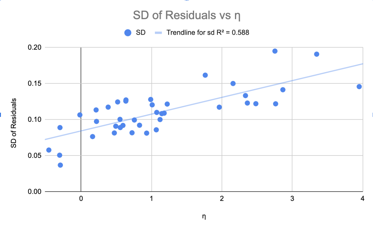
To answer this question, we investigated the relationship between \(\eta _k\) and the residuals, the difference between the actual outcomes and the model predictions, for each student on corresponding KCs. Particularly, we investigated ds99 dataset, where \(\eta _k\) ranges from -0.46 to 3.95 (\(\mu =1.12\)). Let’s first look at the \(h_{ik}\) variables. When the KC has a strong variance for the interactions, which means some students are really strong while some students are really weak on the KC, we will also expect a high variance for \(h_{ik}\) of that KC. In contrast, when the student-KC interactions have a weak variance, \(h_{ik}\) will also be expected to have a low variance. As a result, \(\eta _{k}\) should be correlated with the variance of the corresponding student-KC interactions. The result from the real-student data, as shown in Fig. 1, supports this hypothesis and shows that the variance of the residuals and \(\eta _{k}\) are in fact correlated.
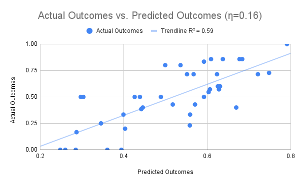
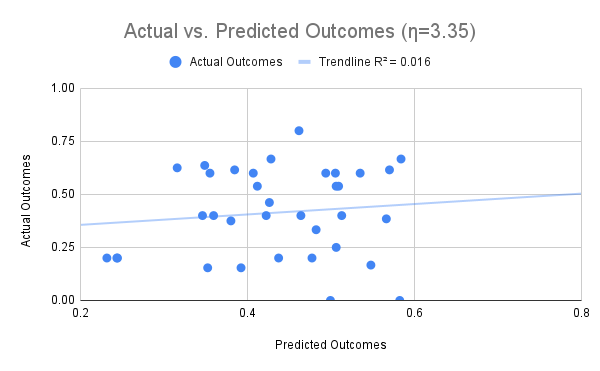
Consequently, the \(\eta _{k}\) can be interpreted as representing the variance of student-KC interactions of the associated KC. In other words, when \(\eta _{k}\) is high, some students are really good at the KC while other students are not. For example, number-letter is a KC with a relatively high \(\eta _{k}\) from the English Article Tutor. The number-letter KC describes a skill that involves selecting an English article (i.e. "a" or "an") to fill in the blank. Examples of problems with number-letter KC are "This is the first time that I’ve received ___ ’99’ on a test." or "My name begins with ___ ’L’.". Some, perhaps otherwise struggling, students may learn this skill faster because they happen to focus on the sound of the letter in the following noun and whether it is a vowel or consonant sound. Other, perhaps otherwise good, students may learn this skill slower because they focus on the written letter and whether it is a vowel or consonant. This latter encoding sometimes works, so it is non-trivial to reject in early induction if a learner thinks of it, However, it produces errors and slows down learning overall. On the other hand, when \(\eta _{k}\) is low, most students are relatively similarly good at that given KC, so the differences in their performance will depend on their overall characteristics, such as student intercepts (prior knowledge). The corollary of this finding is that when \(\eta _{k}\) is low, students are performing as expected from the model’s prediction (Fig. 2) due to the small variances of residuals. Conversely, students are not performing as expected on the KCs when \(\eta _{k}\) is large (Fig. 2). Taken together, these results demonstrate that the \(h\) models are not only better fitting models, but their parameters are also meaningful and interpretable. To illustrate the usefulness of the meaningful interpretations, the above suggests a change in the KC model and associated instruction so that the number-letter KC becomes unambiguous and the variance of students’ learning is reduced.
The implications of an interpretable knowledge tracing model with better predictive power are immense, especially with practical applications. For example, Liu et al. demonstrate that meaningful interpretations of AFM parameters (e.g. learning rates for knowledge components’ slopes) can lead to new scientific insights (e.g. improved cognitive models discovery) and results in useful practical applications (e.g. an intelligent tutoring system redesign) [7]. Similarly, our work has many potential practical applications, such as improved ITS design, better student tracing, and overall improvements to the use of model parameters to make decisions about student learning and mastery.
6. CONCLUSIONS AND FUTURE WORK
In this work, we argued that models with high prediction accuracy do not necessarily exhibit meaningful parameter estimates, which are important for scientific and practical applications. We demonstrated our claim in the context of PFA using both synthetic data and real-student data. The result supported our hypothesis that while PFA is a better fitting model compared to AFM, its parameters’ interpretation is ambiguous. Further, we proposed new models AFMh and PFAh, introducing a success-history variable (\(h_k\)) designed to capture student-KC interactions, to the existing models. We evaluated their capabilities also with synthetic data and real-student data and demonstrated that the new models are both more interpretable and better fitting compared to PFA.
While \(h_k\) works reasonably well as a proxy of student-KC interactions, in future work it might be important to test a model with straightforward student:KC interaction terms; though, there might be a possibly intractable number of parameters. In addition, other possible configurations of \(h_k\) variables could be interesting to experiment with, such as formulating \(h_k\) to be centered at 0 instead of 0.5 or using logarithmic form.
7. ACKNOWLEDGEMENTS
The author(s) disclosed the following financial support for the research, authorship, and/or publication of this article: The preparation of this manuscript was partially supported by National Science Foundation grant #2301130.
8. REFERENCES
- V. Aleven, B. M. McLaren, J. Sewall, and K. R. Koedinger. The cognitive tutor authoring tools (ctat): Preliminary evaluation of efficiency gains. In Intelligent Tutoring Systems: 8th International Conference, ITS 2006, Jhongli, Taiwan, June 26-30, 2006. Proceedings 8, pages 61–70. Springer, 2006.
- H. Cen, K. Koedinger, and B. Junker. Learning factors analysis–a general method for cognitive model evaluation and improvement. In International conference on intelligent tutoring systems, pages 164–175. Springer, 2006.
- K. R. Koedinger, R. S. Baker, K. Cunningham, A. Skogsholm, B. Leber, and J. Stamper. A data repository for the edm community: The pslc datashop. Handbook of educational data mining, 43:43–56, 2010.
- K. R. Koedinger, P. F. Carvalho, R. Liu, and E. A. McLaughlin. An astonishing regularity in student learning rate. Proceedings of the National Academy of Sciences, 120(13):e2221311120, 2023.
- K. R. Koedinger, A. T. Corbett, and C. Perfetti. The knowledge-learning-instruction framework: Bridging the science-practice chasm to enhance robust student learning. Cognitive science, 36(5):757–798, 2012.
- K. R. Koedinger, J. C. Stamper, E. A. McLaughlin, and T. Nixon. Using data-driven discovery of better student models to improve student learning. In Artificial Intelligence in Education: 16th International Conference, AIED 2013, Memphis, TN, USA, July 9-13, 2013. Proceedings 16, pages 421–430. Springer, 2013.
- R. Liu and K. R. Koedinger. Closing the loop: Automated data-driven cognitive model discoveries lead to improved instruction and learning gains. Journal of Educational Data Mining, 9(1):25–41, 2017.
- C. Maier, R. S. Baker, and S. Stalzer. Challenges to applying performance factor analysis to existing learning systems. In Proceedings of the 29th International Conference on Computers in Education, 2021.
- J. Metcalfe. Learning from errors. Annual review of psychology, 68:465–489, 2017.
- A. A. Neath and J. E. Cavanaugh. The bayesian information criterion: background, derivation, and applications. Wiley Interdisciplinary Reviews: Computational Statistics, 4(2):199–203, 2012.
- P. I. Pavlik Jr, H. Cen, and K. R. Koedinger. Performance factors analysis–a new alternative to knowledge tracing. Online Submission, 2009.
- C. Piech, J. Bassen, J. Huang, S. Ganguli, M. Sahami, L. J. Guibas, and J. Sohl-Dickstein. Deep knowledge tracing. Advances in neural information processing systems, 28, 2015.
- N. Rachatasumrit, P. F. Carvalho, S. Li, and K. R. Koedinger. Content matters: A computational investigation into the effectiveness of retrieval practice and worked examples. In International Conference on Artificial Intelligence in Education, pages 54–65. Springer, 2023.
- N. Rachatasumrit and K. R. Koedinger. Toward improving student model estimates through assistance scores in principle and in practice. International Educational Data Mining Society, 2021.
- R. M. Schmidt. Recurrent neural networks (rnns): A gentle introduction and overview. arXiv preprint arXiv:1912.05911, 2019.
- D. Weitekamp, Z. Ye, N. Rachatasumrit, E. Harpstead, and K. Koedinger. Investigating differential error types between human and simulated learners. In Artificial Intelligence in Education: 21st International Conference, AIED 2020, Ifrane, Morocco, July 6–10, 2020, Proceedings, Part I 21, pages 586–597. Springer, 2020.