Fully Latent Principal Stratification with Misspecified Measurement Models in Intelligent Tutoring Systems

Pei, Yanping; Sales, Adam; Kang, Hyeon-Ah; Whittaker, Tiffany

doi:10.5281/zenodo.15870181

Yanping Pei

Worcester Polytechnic Institute

ypei@wpi.edu

Adam C. Sales

Worcester Polytechnic Institute

asales@wpi.edu

Hyeon-Ah Kang

University of Texas, Austin

hkang@austin.utexas.edu

Tiffany A. Whittaker

University of Texas, Austin

t.whittaker@austin.utexas.edu

ABSTRACT

Fully-Latent Principal Stratification (FLPS) offers a promising approach for estimating treatment effect heterogeneity based on patterns of students’ interactions with Intelligent Tutoring Systems (ITSs). However, FLPS relies on correctly specified models. In addition, multiple latent variables, such as ability, participation, and epistemic beliefs, can influence the effect of an ITS. Consequently, any attempt to model the latent space will inevitably involve some misspecification. In this paper, we extend prior work by investigating a more realistic scenario: assessing the impact of model misspecification on the estimation of the Local Average Treatment Effect (LATE) using simulated data. Our simulation setup is grounded in a real Randomized Controlled Trial (RCT) of Cognitive Tutor Algebra 1, an intelligent tutoring platform. This approach minimizes subjective parameter specification by relying on data-driven methods, effectively mimicking real RCT data. Our analysis reveals that FLPS remains robust in estimating LATE even under latent variable misspecification—specifically when two latent variables are used in data simulation while only a single latent variable is used in FLPS estimation. This holds regardless of whether the true LATE is zero or nonzero. These findings highlight FLPS’s resilience to certain model misspecifications, reinforcing its applicability in real-world educational research.

Keywords

User Modeling, Causal Inference, Randomized Controlled Trials

1. INTRODUCTION

As educational technology (EdTech) grows in prominence, so does the urgency to test the efficacy of computer-based learning tools in the field. To answer this need, education researchers have conducted a large number of randomized controlled trials (RCTs) that generate high-quality evidence of EdTech effectiveness [5, 14, 11, 1]. The most important policy goal of these studies is to estimate the average effect of providing access to the products or programs under study.

Nevertheless, these effects are only the beginning of the story—the effectiveness of an educational intervention (one supposes) hinges entirely on how students and teachers actually use it. Fortunately, EdTech RCTs produce, almost as a by-product, rich and detailed information on this very question in the form of student log data. However, discerning important patterns in log data and linking those patterns with varying program effectiveness present serious statistical challenges.

Fully-Latent Principal Stratification (FLPS) [8, 9] may provide a way forward. FLPS combines flexible measurement modeling to identify patterns in log data with rigorous causal analysis. Researchers have used FLPS to estimate the extent to which EdTech effects vary with students’ propensities to master skills (or, conversely, to wheel-spin) [16], game the system [18], receive feedback [9], or re-try problems [17].

Unfortunately, FLPS relies heavily on several strong parametric assumptions– most importantly, that models of students’ behavior and outcomes are correctly specified. Moreover, these assumptions are often difficult or impossible to test. Hence, there is a crucial need for evidence on the impact of model misspecification in FLPS—what types of model misspecification pose the greatest threat? What types of misspecification are innocuous?

This paper is the first attempt at answering those questions: preliminary findings from a simulation study of model misspecification. While the study includes misspecification of models of both student usage and outcomes, we focus on the former. In particular, we investigate the scenario in which a multidimensional latent variable drives students’ experiences, but the FLPS measurement model includes only one dimension. Like [4] and [10], our simulation draws as much as possible from real data—in particular, the outcomes and covariates, as well as the parameters for the measurement model, are all drawn from the Cognitive Tutor Algebra 1 effectiveness trial [12]. In the four scenarios we simulated, the causal estimates performed well, despite model misspecification.

The following section reviews necessary background material, including potential outcomes, FLPS, and item response theory. Section 3 describes our simulation design based on real data, with results in Section 4. Section 5 concludes.

2. BACKGROUND

2.1 Fully-Latent Principal Stratification (FLPS)

Principal stratification (PS) is a causal inference method, used to adjust results for post-treatment covariates, grounded in the potential outcomes framework (Rubin, [15]).

2.1.1 Randomized Controlled Trial (RCT)

Consider an experiment with $N$ participants, indexed as $i = 1,2,...,N$. Each participant can be assigned to either treatment or control arm at random, and we denote $Z_{i}$ following Bernoulli distribution be the $i$ th participant’s treatment assignment, that is,

\begin{align} Z_{i} &\perp \!\!\!\perp Z_{j}, \quad i \neq j \\ \notag P(Z_{i} = t) &= p_{i}^t (1-p_{i})^{1-t}, \quad t \in \{0, 1\} \end{align}

where $Z_{i} = 1$ when the $i$ th participant is assigned to treatment arm and $Z_{i} = 0$ when control arm. Furthermore, we observe outcomes $Y_{i}$ and $q$-dimensional baseline covariates $\mathbf {X}_{i}$ besides treatment assignment $Z_{i}$ for each participant.

Assume each participant has two nonrandom potential outcomes– treated potential outcomes $t_{i}$ and control potential outcomes $c_{i}$. We can write observed outcomes $Y_{i}$ as

\begin{equation} Y_{i} = Z_{i}t_{i} + (1-Z_{i})c_{i} \end{equation}

Individual Treatment Effect (ITE) $\tau _{i}$ can be written as

\begin{equation} \tau _{i} = t_{i} - c_{i} \end{equation}

ITEs are unidentified due to $t_{i}$ and $c_{i}$ cannot be observed simultaneously; instead, causal research tends to focus on aggregate treatment effects, such as Average Treatment Effect (ATE) $E(\tau ) = E(Y^{t}) - E(Y^{c})$ or Local Average Treatment Effect (LATE) $E(\tau | \mathbf {X} = \mathbf {x})$.

2.1.2 Principal Stratification (PS)

Principal stratification (Frangakis $\& $ Rubin, [6]) provides a framework for identifying underlying subgroups and estimating causal effects within them. These strata are defined based on variables that may themselves be influenced by treatment assignment. Let $M_{i}$ represent a measure of subject $i$’s implementation, exposure, or compliance with an intervention. For example, in an RCT evaluating a high school where Cognitive Tutor for Algebra 1 (CTA1) is assigned at random, $M_i$ could indicate whether student $i$ use CTA1. In an RCT assessing a behavioral intervention conducted over multiple sessions, $M_{i}$ might represent the number of sessions student $i$ attended. If section difficulty, denoted by $\textit {diff}_{j}$, is considered, we use $M_{ij}$ to account for subject $i$’s implementation, exposure, or compliance in section $j$.

Assume that $M$ has two non-random potential outcomes: $m^{t}$ under the treatment condition and $m^{c}$ under the control condition. For example, we might ask whether student $i$ would use a particular feature of CTA1 if assigned to the treatment group or how many sections student $i$ would attend if randomized to receive the behavioral intervention. Here, we focus on the "one-way noncompliance" case, where $m^{c}$ is either undefined or remains constant for subjects assigned to the control group. For subjects randomized to the treatment arm, $M$ is observed as $m^{t}$, while for those in the control arm, $m^{t}$ is unobserved but still well-defined.

The goal of PS is to estimate the LATE [3]:

\begin{align} \tau (m) &= E(\tau | M = m^{t}) \\ \notag &= E(t - c | M = m^{t}) \\ \notag &= E(t | M = m^{t}) - E(c | M = m^{t}) \end{align}

Classical PS estimates the LATE by defining strata based on the measurement $M$. However, it assumes that $M$ is a single, error-free measurement. In practice, $\mathbf {M}$ is often multidimensional. Let $\mathbf {m}_{i}$ represent the set of measurements for subject $i$, defined as

\begin{equation} \mathbf {m}_i \equiv \{m_{i1}, m_{i2}, \dots , m_{iJ_{i}} \} \end{equation}

where $J_{i}$ denotes the number of measurements available for subject $i$.

One approach to incorporating multidimensional measurements $\mathbf {M}$ is to aggregate them using a pre-specified function, such as the sample mean $\bar {m}$. This aggregate can then be used as a unidimensional intermediate variable, allowing us to stratify based on its potential values $\bar {m}^{t}$. However, this approach overlooks measurement error in the aggregate, which becomes more problematic when the number of measurements varies across individuals, leading to differential error. Additionally, accounting for treatment effect variation across multiple variables can impose high demands on estimation and modeling. As a result, when multivariate data is measured with error, traditional PS becomes challenging to implement.

2.1.3 Fully-Latent PS (FLPS)

Unlike classical PS, FLPS approach models the measurement process via setting the distribution of $\mathbf {M}$, denoted as $P(\mathbf {m}_i \mid \boldsymbol {\eta }_i^t)$, where $\boldsymbol {\eta }_{i}^{t}$ is a subject-level latent trait capturing the construct of interest. We then assume that $\boldsymbol {\eta }_{i}^{t}$ encapsulates all relevant information about the potential outcomes reflected in $\mathbf {m}$, leading to the conditional independence assumption:

\begin{equation} \{t_{i}, c_{i}\} \perp \!\!\!\perp \mathbf {M}_{i} \mid \boldsymbol {\eta }_{i}^{t}, \mathbf {X}_{i} \end{equation}

The causal estimand in FLPS, $\tau (\boldsymbol {\eta }^{t}) \equiv E(\tau |\boldsymbol {\eta }^{t})$, represents the LATE for individuals who would follow the intervention strategy as $\boldsymbol {\eta }^{t}$ if assigned to the treatment arm.

When the latent trait $\boldsymbol {\eta }^{t}$ is observed, the joint density of the data can be expressed as:

\begin{align} p(Y, \boldsymbol {\eta }^{t}, \mathbf {m} \mid \mathbf {X}, Z=1) &= P(t \mid \boldsymbol {\eta }^{t}, \mathbf {X}) p(\mathbf {m} \mid \boldsymbol {\eta }^{t}) p(\boldsymbol {\eta }^{t} \mid \mathbf {X}), \\ \notag p(Y, \boldsymbol {\eta }^{t}, \mathbf {m} \mid \mathbf {X}, Z=0) &= p(c \mid \boldsymbol {\eta }^{t}, \mathbf {X}) p(\boldsymbol {\eta }^{t} \mid \mathbf {X}). \end{align}

where $p(t, \boldsymbol {\eta }^{t}, \mathbf {m} \mid \mathbf {X})$ and $p(c, \boldsymbol {\eta }^{t}, \mathbf {m} \mid \mathbf {X})$ represent the potential outcome models, $p(\mathbf {m} \mid \boldsymbol {\eta }^{t})$ corresponds to the measurement model, and $p(\boldsymbol {\eta }^{t} \mid \mathbf {X})$ characterizes the latent trait as a function of the covariates.

The latent trait $\boldsymbol {\eta }^{t}$ is unobserved in both the treatment and control arms, but the data structure differs between them. In the treatment arm, the model for $\boldsymbol {\eta }^{t}$ incorporates both measurements $\mathbf {m}$ and covariates, whereas in the control group, it includes only covariates.

Let $\boldsymbol {\theta }$ be a vector of parameters in the FLPS model. This includes $\tau _{0}$ and $\tau _{1}$, which represent the principal effects (i.e., intercept and slope), $\omega $, which captures the effect of the latent factor, and $\boldsymbol {\beta }$ and $\boldsymbol {\gamma }$, which model the covariate effects on $\boldsymbol {\eta }^{t}$ and $Y$, respectively. Assuming that the observed data are independently and identically distributed given $\boldsymbol {\theta }$, $Z$, and $\mathbf {X}$, the factorization in Equation ($7$) leads to the following likelihood function for $\boldsymbol {\theta }$:

\begin{align} & L(\boldsymbol {\theta } \mid Y, Z, \mathbf {X}, \mathbf {m}): \\ \notag & \prod _{i: Z_{i} = 1} \int p(Y_{i} \mid Z_{i}, \boldsymbol {\eta }_{i}^{t}, \mathbf {X}_{i}, \boldsymbol {\theta }) p(\mathbf {m}_{i} \mid \boldsymbol {\eta }_{i}^{t}, \boldsymbol {\theta }) p(\boldsymbol {\eta }_{i}^{t} \mid \mathbf {X}_{i}, \boldsymbol {\theta }) d\boldsymbol {\eta }_{i}^{t} \\ \notag & \cdot \prod _{i: Z_{i} = 0} \int p(Y_{i} \mid Z_{i}, \boldsymbol {\eta }_{i}^{t}, \mathbf {X}_{i}, \boldsymbol {\theta }) p(\boldsymbol {\eta }_{i}^{t} \mid \mathbf {X}_{i}, \boldsymbol {\theta }) d\boldsymbol {\eta }_{i}^{t}. \end{align}

In Equation ($8$), the first product corresponds to individuals in the treatment arm ($Z_{i} = 1$), where both outcome and measurement models are included. The second product represents individuals in the control group ($Z_{i} = 0$), where only the outcome and latent trait models are considered. The outcome model $p(Y_{i} \mid Z_{i}, \boldsymbol {\eta }_{i}^{t}, \mathbf {X}_{i}, \boldsymbol {\theta })$ describes how $Y_{i}$ depends on covariates ($\mathbf {X}_{i}$), the latent trait ($\boldsymbol {\eta }_{i}^{t}$), and treatment ($Z_{i}$). The measurement model links $\mathbf {m}$ to $\boldsymbol {\eta }^{t}$, which varies with $\mathbf {X}$.

Since the integrals in Equation (8) are intractable, direct likelihood maximization is not feasible. Instead, we use a Bayesian Markov Chain Monte Carlo (MCMC) approach to approximate the posterior distribution of $\theta $, following prior FLPS research [16]. Specifically, this study employs No-U-Turn Sampling (NUTS), the default sampler in Stan. NUTS is an adaptive variant of the Hamiltonian Monte Carlo (HMC) method and has been shown to be computationally efficient for estimating correlated parameters [7].

2.2 Item Response Theory (IRT)

Item Response Theory (IRT) models the relationship between unobservable traits, such as knowledge or attitudes, and observed responses to test items, placing both traits and items on a continuous latent scale. In FLPS, we construct the measurement model using IRT, where each measurement is characterized by an item parameter $\boldsymbol {\zeta }_j$, which may be a vector, associated with measurements from each unique item that students interact with, $\mathbf {M}_{j}$ , and a scalar subject-level parameter $\eta _{i}^{t}$.

Assuming local independence, the measurements for a given subject $i$ are conditionally independent, given $\boldsymbol {\zeta }$ and $\eta _{i}^{t}$. Formally, for $j \neq j' \in \mathcal {J}_i$, we have:

\begin{equation} M_{ij} \perp \!\!\!\perp M_{ij'} \mid \boldsymbol {\zeta }, \eta _{i}^{t}, \end{equation}

where $\boldsymbol {\zeta }$ is a vector of item parameters across all items. Then the measurement model is completely specified by a model for each measurement occasion $M_{ij}$.

2.2.1 Rasch Model

For binary responses $M_{ij}$, the most fundamental measurement model is the Rasch model [13], which specifies the probability of a correct response ($M_{ij} = 1$) as:

\begin{equation} \phi _{ij} = P(M_{ij} = 1 \mid \eta _{i}^{t}, d_{j}) = logit^{-1} (\eta _{i}^{t} + d_{j}), \end{equation}

where $\textit {logit}^{-1}(x) = \frac {1}{1 + e^{-x}}$, and $\zeta _{j} = d_{j}$ represents a scalar intercept parameter.

We assume that $\eta _{i}^{t}$ follows a normal distribution given the covariates $\mathbf {x}_{i}$:

\begin{equation} \eta _{i}^{t} \mid \mathbf {x}_{i} \sim \mathcal {N}(\beta _{0} + \beta ' \mathbf {x}_{i}, \sigma _{\eta }^2), \end{equation}

where $\boldsymbol {\beta }$ is a coefficient vector, and $\sigma _{\eta }^2$ represents the variance.

Additionally, we assume that $Y_{i}$ is normally distributed conditional on $Z_{i}$, $\mathbf {x}_{i}$, and $\eta _{i}^{t}$:

\begin{equation} Y_{i} \mid Z_{i}, \eta _{i}^{t},\mathbf {x}_{i} \sim \mathcal {N}(\gamma _{0} + \boldsymbol {\gamma }'\mathbf {x}_{i} + \omega \eta _{i}^{t} + Z_{i}(\tau _{0}+\tau _{1}\eta _{i}^{t}), \sigma _{Y}^{2}) \end{equation}

Equation (11) implies a linear model for the expected treatment effect as of function of $\eta ^{t}$: $E(Y \mid Z=1, \eta ^{t}) - E(Y \mid Z=0, \eta ^{t}) = \tau _{0} + \tau _{1}\eta ^{t}$.

Overall, the parametric FLPS models consist of two main components. The first is a measurement submodel, $f(M \mid \eta ^{t}, \boldsymbol {\zeta })$, as described in Equation (10) assuming local independence. The second component involves linear-normal models. Specifically, Equation (11) defines $\eta ^{t}$ as a normal variable conditioned on $\mathbf {x}$, with parameters $\boldsymbol {\beta }$ and $\sigma _{\eta }^2$. Similarly, Equation (12) models $Y$ as a normal variable dependent on $\mathbf {x}$, $Z$, and $\eta ^{t}$, characterized by the parameters $\boldsymbol {\gamma }$, $\omega $, $\tau _{0}$, $\tau _{1}$, and $\sigma _{Y}^{2}$.

2.2.2 Two-Parameter Logistic (2-PL) Model

The Two-Parameter Logistic (2PL) model defines the item response function as:

\begin{equation} P(M_{ij} = 1 \mid \eta _{i}^{t}, a_{j}, d_{j}) = logit^{-1} (a_{j} \eta _{i}^{t} + d_{j}), \end{equation}

where $M_{ij} \in \{0,1\}$ represents the response of subject $i$ to item $j$, and $\eta _{i}^{t}$ denotes the subject’s latent trait level. The parameters $a_{j}$ and $d_{j}$ correspond to the item’s discrimination (slope) and difficulty (intercept), respectively. If $a_{j}$ is fixed at one, the model simplifies to the Rasch model.

For simplicity, we used the Rasch model to simulate the data and employed both the Rasch and 2-PL models as measurement models in the FLPS calculation. This setup ensures model misspecification, as the simulated data includes two latent variables, $\eta _{1}^{t}$ and $\eta _{2}^{t}$, while the FLPS model only accounts for a single latent variable, $\eta ^{t}$. In future analyses, we can also explore other measurement models to handle polytomous responses, such as Generalized Partial Credit Model (GPCM) and the Graded Response Model (GRM).

3. SIMULATION DATA BASED ON CTA1

3.1 Cognitive Tutor Algebra 1 (CTA1)

As one of the first widely adopted intelligent tutoring systems, the Cognitive Tutor[2], first developed at Carnegie Mellon University and later managed by Carnegie Learning, has since been replaced by Carnegie Learning’s Mathia program. Our simulated data is based on a real randomized effectiveness study conducted by the RAND Corporation between 2007 and 2009, which is funded by the U.S. Department of Education.

Around $25,000$ students across $73$ high schools and $74$ middle schools in seven states across two school years are included in this study. Schools were paired based on some vital factors including school level (middle or high), size, district, and prior achievement at first, and randomized to either use CTA1 or usual curriculum in the next two school years. Students’ standardized algebra $1$ posttest score in both the treatment schools and matched controls is what we interested in. J. F. Pane et al. [12] reported that estimated treatment effects of $0.1$ with standard deviations ($95\%$ CI: $-0.3$ to $0.1$) in year $1$ while $0.21$ with standard deviations ($95\%$ CI: $0.01$ to $0.41$) in year $2$ within the high school stratum.

We focus on students in the treatment arm of the CTA1 experiment, recognizing that their level of commitment to implementing the intervention may vary. To refine the dataset, we include only students who either mastered or were promoted in Algebra 1, excluding those enrolled in other curricula. Specifically, we define mastered as students who successfully completed all required coursework and met the mastery criteria, while promoted refers to students who advanced to the next level despite not fully meeting mastery requirements.

To ensure reliable posttest scores and preserve variation in mastery status, we exclude sections with fewer than 100 students and those in which all students mastered. After filtering, we group the data by student ID and section, summarizing mastery status.

Table 1 provides a detailed description of the features used in our analysis.

Table 1: Description of Used Variables
Feature	Description
master	Whether the student mastered the skill (binary)
xirt	Student’s prior performance score
race	WhiteAsian \| BlackMulti \| HispAIAN
sex	F \| M
spec	typical \| speced \| gifted
field_id	Student’s ID
section	Section ID

3.2 Data Simulation

To ensure that the simulated data closely mirrors the structure and characteristics of the original CTA1 experiment, we employ a data-driven simulation approach grounded in the experimental design. This method minimizes reliance on arbitrary parameter settings and enhances the realism of the simulated data used for FLPS estimation.

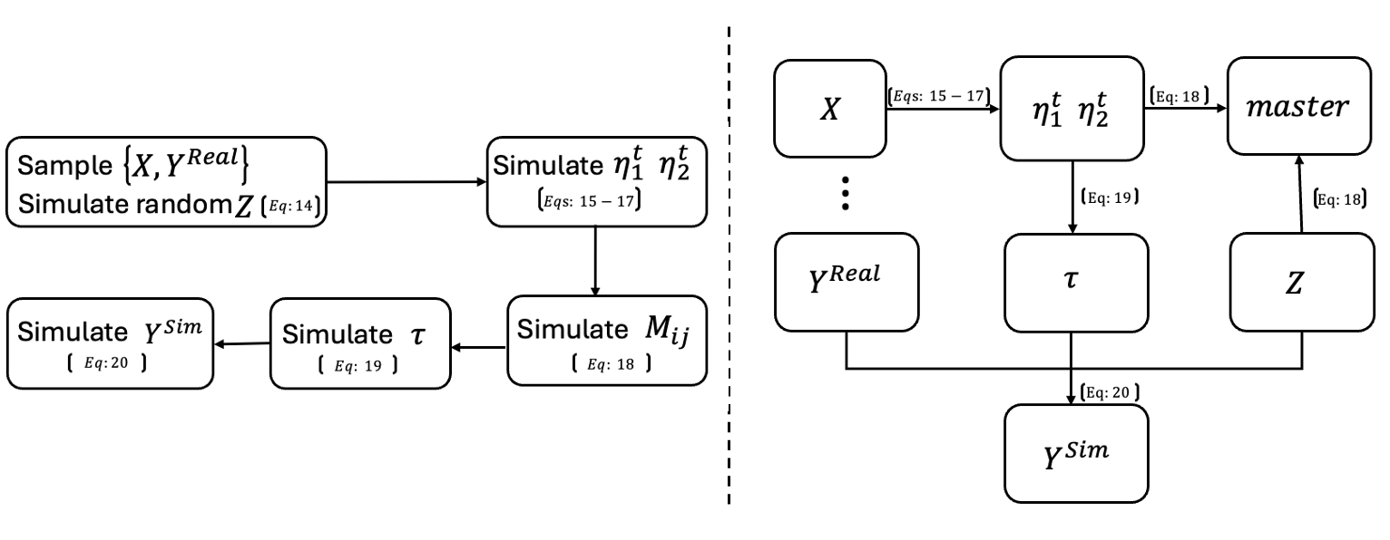
Figure 1 provides an overview of the simulation workflow and the dependencies among key variables. The left panel outlines the sequential steps taken to construct the simulated dataset, with equation references provided for each step. The right panel illustrates the structural relationships among variables used in the simulation. Together, these diagrams clarify the generative process and guide the reader through the logic of the simulation procedure. Each step is discussed in detail in the following sections.

Flowchart of FLPS steps — Figure 1: Overview of Data Simulation Workflow and Variable Dependencies. The left panel outlines the simulation steps, with equation references provided for reproducibility. The right panel depicts the structural relationships among covariates ($\mathbf {X}$), latent traits ($\eta _1^t, \eta _2^t$), treatment assignment ($Z$), mastery status, and outcomes ($Y^{Sim}$).

3.2.1 Random Sampling and Treatment Assignment

To evaluate the robustness of FLPS under model misspecification in a simulation study, we generated data consisting of covariates $\mathbf {X}$, treatment assignment $Z$, a binary variable $master$ indicating whether a student mastered a specific section, and the outcome variable $Y$, representing the posttest score.

We begin by randomly selecting $n = 2000$ students from the CTA1 treatment arm, which contains a total of $N = 5960$ students. This sample size strikes a balance between computational speed and representativeness. For each selected student, we observe covariates $\mathbf {X}$ and the observed real outcome $Y^{Real}$.

The simulated treatment assignment $Z^{Sim}$ is generated independently for each student using a Bernoulli distribution with probability $p = 0.5$, such that

\begin{align} Z_i^{Sim} &\perp \!\!\!\perp Z_j^{Sim} \quad i \neq j \\ \notag P(Z_i^{Sim} = z) &= p^z (1-p)^{1-z} \quad \text {where } z \in \{0, 1\} \end{align}

3.2.2 Simulating Latent Variables $\boldsymbol {\eta }^{t}$

We define the latent variables as proxies for students’ intentions to engage with the treatment intervention. These latent traits are determined by population-level covariate coefficients and each student’s individual covariate values. Specifically, the latent variables $\eta _{1}^{t}$ and $\eta _{2}^{t}$ are simulated as follows:

\begin{equation} \eta _{1}^{t} = \mathbf {X} \cdot coefs + \epsilon \end{equation}

\begin{equation} cor(\eta _{1}^{t}, \eta _{2}^{t}) = \rho \end{equation}

where $\mathbf {X}$ is the design matrix derived from the sampled data, coefs denotes the population-level covariate coefficients, and $\epsilon \sim \mathcal {N}(0, 1)$ is standard normal noise. We explore two values of the correlation parameter, $\rho = 0.5$ and $\rho = 0.2$.

To ensure that the simulated data reflect patterns observed in the real CTA1 RCT, we estimate the coefficient vector coefs using a generalized linear mixed model (GLMM) with a logistic link function, fitted on the population data. The fitted model is given by:

\begin{align} P(master = 1) &= logit^{-1} \Big ( 3.3601 + 0.8402 \cdot xirt \\ \notag &\quad - 0.5588 \cdot raceBlackMulti \\ \notag &\quad - 0.6624 \cdot raceHisPAIAN + 0.5134 \cdot sexM \\ \notag & \quad - 0.6016 \cdot specspeced + 0.1508 \cdot specgifted\\ \notag &\quad + u_{field\_id} + v_{section} \Big ) \end{align}

where $u_{field\_id} \sim \mathcal {N}(0, 1.328)$ and $v_{section} \sim \mathcal {N}(0, 9.351)$ represent the random intercepts for field_id and section, respectively.

Table 2 displays a subset of section-level difficulty estimates, which are incorporated into the simulation of the latent variables $\eta _{1}^{t}$ and $\eta _{2}^{t}$. ¹

Table 2: Subset of Section-Level Difficulty Estimates
Section	Difficulty Estimate
centraltendency1	1.0889
centraltendency2	-1.3397
centraltendency3	-1.8160
centraltendency4	-0.4317
cta1012	0.1232
cta1013	-2.0371

3.2.3 Simulating the Rasch Measurement Model

Given the simulated latent variables and treatment assignments, we define the latent data structure using a Rasch measurement model applied to the simulated treatment arm. The probability that student $i$ successfully masters section $j$ is modeled as:

\begin{equation} P(M_{ij} = 1) = logit^{-1} \left [ \alpha \cdot \eta _{1i}^{t} + (1 - \alpha ) \cdot \eta _{2i}^{t} - diff_{j} \right ] \end{equation}

where $M_{ij}$ indicates whether student $i$ successfully masters section $j$, $\eta _{1i}^{t}$ and $\eta _{2i}^{t}$ represent latent intentions, and $diff_{j}$ denotes the difficulty level of section $j$.

To align the simulated mastery outcomes with those observed in the real data, we apply a post-processing adjustment denoted as fakeOut, ensuring that the total number of mastered sections in the simulated data approximates that in the real dataset, i.e., $\sum _{j} M_{ij}^{Sim} \approx \sum _{j} M_{ij}^{Real}$, where $M_{ij}^{Real}$ corresponds to observed mastery statuses in the original study.

3.2.4 Simulating Treatment Effect $\tau $

We assume that the treatment effect can either be influenced by the latent variables defined earlier or be absent. We simulate the treatment effect $\tau $ as follows:

\begin{equation} \tau = \begin {cases} 0 & \textit {LATE} = 0 \\ \tau _0 + \tau _1 \cdot \eta _{1}^{t} & \textit {LATE Influenced by $\eta $} \end {cases} \end{equation}

where $\tau _0$ is set as $\tau _0 = LATE - \tau _1 \cdot \bar {\eta }_{1}^{t}$ to ensure that the LATE remains consistent. We set $LATE = 0.3$ and $\tau _1 = 0.2$.

3.2.5 Simulating Outcomes $Y^{Sim}$

We simulate the outcome of interest, $Y_i^{Sim}$, based on the observed outcome $Y_i^{Real}$, simulated treatment assignment $Z_i^{Sim}$, and individual treatment effect $\tau _i$, as follows:

\begin{equation} Y_i^{Sim} = Y_i^{Real} + Z_i^{sim} \cdot \tau _i \end{equation}

Finally, we remove sections where mastery status does not vary and merge the student-level data with log data to ensure the proper format for FLPS estimation.

4. IMPLEMENTATION AND RESULTS

We focus on examining how the treatment effect interacts with the latent variables. Specifically, we consider two LATE scenarios:

Scenario 1: Constant Treatment Effect

\begin{equation} \tau _{i} = 0 \quad \quad i \in \{1,2,\dots , n\} \end{equation}

where all units in the simulated sample receive no treatment effect.

Scenario 2: Latent Variable-Dependent Treatment Effect

\begin{equation} \tau _{i} = \tau _{0} + \tau _{1} \cdot \eta _{1}^{t} \end{equation}

where the treatment effect varies across units based on their latent variable $\eta _{1}^t$.

Table 3 provides an overview of the manipulated factors, condition levels, and the distribution of randomly generated parameters.

Table 3: Simulation Design
Condition	Simulation Factor	Notation
Manipulation	Measurement model	Rasch & 2-PL
	Treatment effect type	Constant & Latent Variable-Dependent ($\tau $)
	Correlation between latent variables	$cor(\eta _{1},\eta _{2}) = 0.5$ & $cor(\eta _{1},\eta _{2}) = 0.2$
	Contribution of $\eta _{1}^{t}$to $M_{ij}$	$\alpha = 0.9$ & $\alpha = 0.5$
Fixed setup	Sample size	$n = 2000$
	Treatment assignment	$Z \sim Binomial (n, p)$ with $p = 0.5$
	Latent trait distribution	$\eta _{i}^{t} \mid \mathbf {x}_{i} \sim \mathcal {N}(\beta _{0} + \boldsymbol {\beta }' \mathbf {x}_{i}, \sigma _{\eta }^2)$
	Outcome model	$Y_{i} \mid Z_{i}, \eta _{i}^{t}, \mathbf {x}_{i} \sim \mathcal {N}(\gamma _{0} + \boldsymbol {\gamma }' \mathbf {x}_{i} + \omega \eta _{i}^{t} + Z_{i}(\tau _{0}+\tau _{1}\eta _{i}^{t}), \sigma _{Y}^{2})$

The FLPS model parameters were estimated using Stan via the rstan package in R, which implements Hamiltonian Monte Carlo (HMC) sampling. The structural model employed Stan’s default priors (i.e., reference distributions). For Bayesian estimation, we ran four MCMC chains, each with $50,000$ iterations, discarding the first $40,000$ samples as part of the burn-in period. The posterior mean of each parameter was used as its MCMC estimate.

4.1 mirt-Based Latent Trait Evaluation

We use the mirt package in R to evaluate whether the population model used to generate the initial parameters in our data simulation effectively captures the latent traits influencing responses. The results of the fitted models are summarized in Tables 4 and 5.

Table 4: MIRT Model Without Covariate Adjustment
Iteration	Log-Likelihood	Max-Change	Formula
32	-9636.102	0.00006	$y \sim x$

Table 5: MIRT Model With Covariate Adjustment
Iteration	Log-Likelihood	Max-Change	Formula
28	-9573.905	0.00009	$y \sim x$

To further assess model performance, Table 6 compares the models with and without covariate adjustment based on model selection criteria, including Akaike Information Criterion (AIC), Sample-Size Adjusted Bayesian Information Criterion (SABIC), Hannan-Quinn Criterion (HQ), Bayesian Information Criterion (BIC), and log-likelihood. Since lower values indicate better model fit, the covariate-adjusted model (mod_mirt_covariates) outperforms the model without covariates (mod_mirt_without_covariates) across all criteria. Additionally, a likelihood ratio test reveals a significant chi-square statistic ($\chi ^{2} = 124.396, df = 6, p < 0.001$), confirming that the covariate-adjusted model provides a significantly better fit than the model without covariates. These results suggest that incorporating covariates enhances model estimation and improves the representation of the underlying data structure.

Table 6: Comparison of MIRT Models With and Without Covariate Adjustment
Model	AIC	SABIC	HQ	BIC	logLik	$\chi ^{2}$	df	$p$
mod_mirt_without_covariates	19498.21	19670.54	19702.11	20029.39	-9636.102	-	-	-
mod_mirt_covariates	19385.81	19567.30	19600.54	19945.20	-9573.905	124.396	6	<0.001

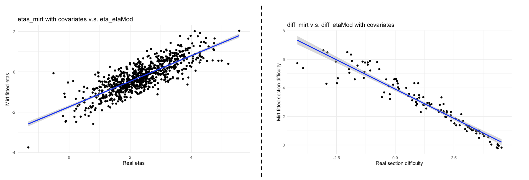
Furthermore, Figure 2 compares the estimated latent traits from the mirt model to the simulated true values. The strong correspondence between the two confirms that the fitted population model with covariates effectively captures the latent trait structure.

Figure 2: Comparison of Estimated and True Latent Trait Values

4.2 Local Average Treatment Effect (LATE)

When conducting causal inference with FLPS, our primary goal is to estimate the LATE. To assess the robustness of FLPS under model misspecification, we run $128$ simulations on Turing for each simulated scenario. Specifically, we examine whether FLPS still provides reliable LATE estimates when the latent variable model used for data simulation differs from the one assumed in estimation. In our data simulation (Section 3), we generate data using a model with two latent variables. However, in the FLPS estimation process, we assume only a single subject-level latent variable. The following Algorithm 1 outlines the FLPS estimation procedure:

Algorithm 1: FLPS Model Estimation
1: Set the number of cores for parallel computation:
mc.cores ← 4
2: Initialize model fitting procedure with FLPS:
3: Attempt to run the FLPS model with the following
inputs:
4: Input Data: data_flps
56:: OTurteacotmmeenVta Vraiarbialbe:le:Y_stirematment_sim
7: Covariates: covariates
8: Latent Variable Model: lvModel
9: Latent Variable Type: rasch
10: Prior Distributions:
11: τ0 ∼ 𝒩(0,1)
12: τ1 ∼ 𝒩(0,1)
113:4: Stanω ∼Sa𝒩mp(0li,n1g) Options:
15: Number of Iterations: 50,000
16: Warmup Iterations: 40,000
17: Number of Chains: 4
18: Thinning Factor: 10
19: Handle errors if model fitting fails
20: Output estimated model parameters

To conserve storage space, we saved only a randomly selected simulation result to present the full model output. However, we retained the model summaries for all simulation runs to ensure the validity of our LATE estimates.

4.2.1 Model Validation Based on a Randomly Selected Simulation Result

Tables 7 and 8 present the results from a randomly selected simulation run, demonstrating that the FLPS estimation performs well for both LATE and latent coefficient estimation. The effective sample size ($n\_{\text {eff}}$) is close to 4000, and the potential scale reduction factor ($Rhat$) is 1, indicating proper convergence.²

Table 7: LATE Estimates on $\tau _{0}$ and $\tau _{1}$
Parameter	Mean	SD	2.5%	25%	50%	75%	97.5%	n_eff	Rhat
$\tau _0$	0.31	0.03	0.25	0.29	0.31	0.33	0.37	3974	1
$\tau _1$	0.20	0.04	0.11	0.17	0.20	0.23	0.29	3964	1

Table 8: LATE Estimates on Covariate Coefficients
Coefficient	Mean	SD	2.5%	25%	50%	75%	97.5%	n_eff	Rhat
xirt	0.72	0.07	0.59	0.67	0.72	0.76	0.85	3995	1
raceBlackMulti	-0.64	0.11	-0.86	-0.71	-0.64	-0.57	-0.43	3701	1
raceHispAIAN	-0.54	0.13	-0.80	-0.63	-0.54	-0.45	-0.29	3963	1
sexM	0.47	0.09	0.29	0.41	0.47	0.54	0.66	4118	1
specspeced	-0.27	0.19	-0.64	-0.40	-0.27	-0.14	0.11	4096	1
specgifted	-0.29	0.24	-0.73	-0.45	-0.29	-0.13	0.18	3875	1

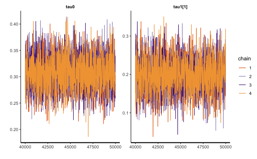
To further assess model convergence and fitting quality, we also visualize the trace plots, as shown in Figure 3. These plots help confirm that the MCMC chains are well-mixed and have reached stationarity.

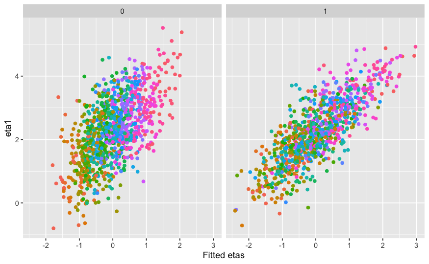
Moreover, Figure 4 illustrates that the fitted latent trait $\eta ^t$ closely matches the true $\eta ^t$, reinforcing the reliability of our model.

Figure 4: Comparison of Estimated Latent Trait ($\eta ^t$) Across Treatment Groups with *xirt* Color-Coded

Given $\eta ^t$, LATE estimation can be computed using the following formula:

\begin{equation} \widehat {LATE} = \hat {\tau }_0 + \hat {\tau }_1 \bar {\eta }_{1}^{t} \label {eq: LATE} \end{equation}

Applying this formula to our results, we obtain LATE $= 0.3060$, which closely aligns with the true value of $0.3$, further validating the accuracy of our estimation. Since by design $E[\eta _1^t]=0$, $\hat {\tau }_0$ may also be taken as an estimate of the LATE.

4.2.2 Model Validation Across All Simulation Runs

We considered four simulation scenarios: two with a constant treatment effect ($LATE = 0$) and two with a latent variable-dependent treatment effect ($LATE = \tau _{0} + \tau _{1}\eta _{1}^{t}$). Within each scenario, we examined two correlation structures.

In the first setting, we set $cor(\eta _{1}^{t}, \eta _{2}^{t}) = 0.5$ and $\alpha = 0.9$, meaning that $\eta _{1}^{t}$ and $\eta _{2}^{t}$ are moderately correlated, with $\eta _{1}^{t}$ contributing 90% to $M_{ij}$. In the second setting, we reduced the correlation to $cor(\eta _{1}^{t}, \eta _{2}^{t}) = 0.2$ and set $\alpha = 0.5$, making the latent traits more distinct. This latter scenario better reflects real-world conditions where latent traits tend to be less correlated.

To assess the robustness of the FLPS model under model misspecification, we evaluate the proportion of true $ \tau $ values and coefficients that fall within the 50% and 95% posterior credible intervals. A well-calibrated model should yield coverage proportions close to 50% and 95%, respectively, indicating its reliability. Table 9 summarizes the posterior credible interval coverage for each simulation scenario, with well-performing proportions highlighted in bold.

Table 9: Posterior Credible Interval Coverage Proportions for Each Simulation Scenario
Simulation Scenario	$\rho = 0.5$ $\alpha = 0.9$				$\rho = 0.2$ $\alpha = 0.5$
	$\tau _0 = \tau _1 = 0$		$\tau _0 = 0.3\quad \tau _1 = 0.2$		$\tau _0 = \tau _1 = 0$		$\tau _0 = 0.3\quad \tau _1 = 0.2$
Posterior CI	50%	95%	50%	95%	50%	95%	50%	95%
$\tau _0$	0.48	0.95	0.45	0.92	0.56	0.94	0.51	0.95
$\tau _1$	0.59	0.93	0.49	0.97	0.57	0.96	0.36	0.82
xirt	0.01	0.06	0.01	0.07	0.00	0.00	0.00	0.00
raceBlackMulti	0.29	0.83	0.36	0.91	0.02	0.25	0.00	0.32
raceHispAIAN	0.27	0.83	0.36	0.89	0.02	0.31	0.02	0.39
sexM	0.19	0.77	0.12	0.62	0.00	0.11	0.00	0.11
specspeced	0.46	0.94	0.41	0.95	0.13	0.61	0.09	0.65
specgifted	0.55	0.98	0.59	0.98	0.59	0.98	0.58	0.97

From Table 9, we observe that the FLPS model performs well, particularly in estimating LATE ($\tau _0$) and in most cases of $\tau _1$, demonstrating its robustness in treatment effect estimation. However, the model is less accurate in estimating the coefficients, likely due to the influence of multiple latent variables. Specifically, the FLPS-estimated latent trait is a weighted combination of the two true latent traits:

\begin{align} \eta _{FLPS} &= \alpha \eta _{1}^{t} + (1-\alpha )\eta _{2}^{t} \\ \notag &= [\alpha + (1-\alpha )\rho ]\gamma X, \end{align}

where $\rho = cor(\eta _{1}^{t},\eta _{2}^{t})$ represents the correlation between the two latent traits. This formulation suggests that the coefficient estimates may be biased by the factor $\alpha + (1-\alpha )\rho $, particularly when the covariate coefficient is large. For example, we observe that the variable xirt has the greatest impact on the measurement master, and it also exhibits the largest bias in the FLPS estimates. In contrast, the variables specspeced and specgifted have a smaller impact on the measurement and correspondingly show less bias in the FLPS estimates.

Moreover, in the first case, where the latent variable correlation is higher ($cor(\eta _{1}^{t}, \eta _{2}^{t}) = 0.5$ and $\alpha = 0.9$), the factor $\alpha + (1-\alpha )\rho $ is 0.95, which is close to 1. This suggests that the FLPS-estimated latent trait is strongly aligned with the primary latent variable, reducing bias in coefficient estimation. In contrast, in the second scenario, where the correlation is lower, $\alpha + (1-\alpha )\rho $ decreases to 0.6, meaning that the estimated latent trait deviates more from the primary latent variable, leading to greater bias. This aligns with the results in the Table 9, where the coverage proportions in the first scenario are closer to the expected values than in the second scenario. Nevertheless, since the primary objective is to estimate LATE ($\tau _{0}$ and $\tau _1$), the FLPS model remains reliable.

Figure 5 presents violin and scatter plots of the estimation error for $\hat {\tau }_0$ and $\hat {\tau }_1$ across four simulation scenarios, where estimation error is defined as the posterior mean minus the true value. The left column represents cases with a constant treatment effect ($\tau _0 = 0, \tau _1 = 0$), while the right column corresponds to cases where the treatment effect depends on latent variables ($LATE = \tau _0 + \tau _1\eta _1^t$ with $\tau _0 = 0.3, \tau _1 = 0.2$). The top row ($\rho = 0.2, \alpha = 0.5$) represents weaker correlation between latent traits, while the bottom row ($\rho = 0.5, \alpha = 0.9$) represents stronger correlation.

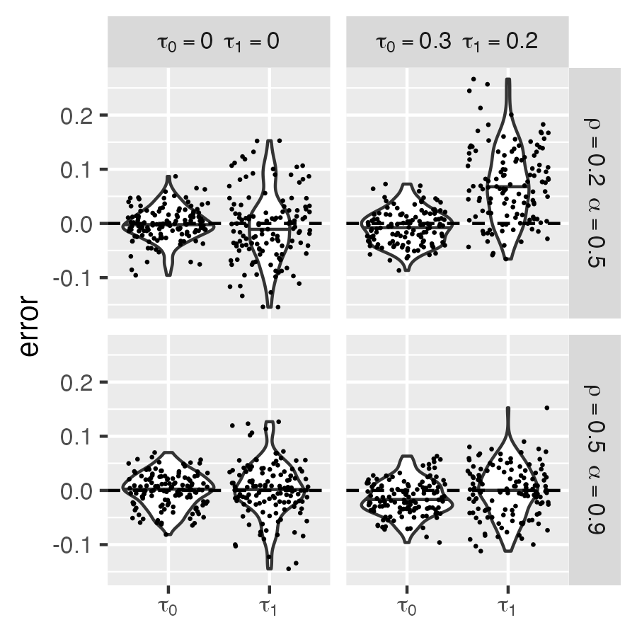
Figure 5: Violin and Scatter Plots of Estimation Error (posterior mean minus population value)

The violin plots indicate that the estimation error for $\hat {\tau }_0$ is well-centered around zero in all cases, suggesting that the FLPS model provides reliable estimates for LATE, even under model misspecification. However, in the latent-variable-dependent treatment effect cases, $\hat {\tau }_1$ exhibits greater variability, particularly in the low-correlation scenario ($\rho = 0.2, \alpha = 0.5$), where the estimation error distribution is wider. In contrast, higher correlation ($\rho = 0.5, \alpha = 0.9$) leads to a tighter error distribution, indicating improved estimation accuracy. Despite increased variation in $\hat {\tau }_1$ when the model is misspecified, its error remains centered around zero, suggesting that the FLPS model still provides an unbiased estimate of $\tau _1$ under these conditions.

Besides, we applied the 2-PL model as the measurement model within the FLPS framework to assess its robustness under model misspecification. When evaluating convergence, we found that MCMC successfully converged in only half of the runs. This suggests that when data is simulated using the Rasch model but estimated with the 2-PL model, convergence issues become more pronounced. One possible explanation is that the 2-PL model introduces an additional discrimination parameter, increasing the complexity of the estimation process. However, the exact cause remains unclear, and further investigation is needed to better understand this issue.

5. DISCUSSION

Our findings suggest that FLPS remains robust in estimating LATE even when the latent variable structure is mis- specified– specifically when two latent variables are used in data simulation, but only one is modeled in estimation. This robustness holds whether the true LATE is zero or nonzero, highlighting FLPS’s practical applicability in real-world educational research. These results are particularly relevant for ITS studies, where multiple latent constructs, such as ability and engagement, influence learning outcomes. Despite simplifying the latent structure, and considerable bias in estimating regression coefficients, FLPS still produces reliable LATE estimates, making it a valuable tool for causal inference in educational settings. Additionally, grounding our simulations in real RCT data enhances the realism of our findings.

The work presented here is preliminary—we will need to investigate a much wider set of scenarios to establish FLPS’s strengths and vulnerabilities. Further evaluation under different forms of model misspecification—such as alternative measurement models (e.g., different IRT models or AI-based approaches for modeling the relationship between $\mathbf {M}$ and $\boldsymbol {\eta }^t$) and varying manually set parameters ($\rho $ and $\alpha $)—will help validate its robustness. Large-scale ITS datasets with well-characterized student traits could also provide deeper insights into FLPS’s real-world effectiveness. Finally, future research should explore strategies to mitigate bias from misspecification, such as hierarchical modeling or sensitivity analyses. Though the work here is preliminary, it is quite encouraging.

In conclusion, while improving model specification enhances LATE estimation—particularly when latent variable correlation is high—FLPS demonstrates resilience to certain misspecifications, making it a promising approach for estimating treatment effect heterogeneity in ITS research. Addressing its limitations through methodological refinements will further improve its reliability and applicability in educational causal inference.

6. ACKNOWLEDGMENTS

The research reported here was supported by the Institute of Education Sciences, U.S. Department of Education, through Grant R305D210036. The opinions expressed are those of the authors and do not represent views of the Institute or the U.S. Department of Education.

7. REPLICATION MATERIALS

Analysis code is available at https://github.com/yanpingPei/FLPS_misspecification_EDM. The CTA1 dataset is not publicly available due to privacy constraints.

8. REFERENCES

C. Abbey, Y. Ma, M. Akhtar, D. Emmers, R. Fairlie, N. Fu, H. F. Johnstone, P. Loyalka, S. Rozelle, H. Xue, et al. Generalizable evidence that computer assisted learning improves student learning: A systematic review of education technology in china. Computers and Education Open, 6:100161, 2024.
J. Anderson, A. Corbett, K. Koedinger, and R. Pelletier. Cognitive tutors: Lessons learned. Journal of the Learning Sciences, 4:167–207, 04 1995.
J. D. Angrist, G. W. Imbens, and D. B. Rubin. Identification of causal effects using instrumental variables. Journal of the American statistical Association, 91(434):444–455, 1996.
A. H. Closser, A. Sales, and A. F. Botelho. Should we account for classrooms? analyzing online experimental data with student-level randomization. Educational technology research and development, 72(5):2865–2894, 2024.
M. Escueta, A. J. Nickow, P. Oreopoulos, and V. Quan. Upgrading education with technology: Insights from experimental research. Journal of Economic Literature, 58(4):897–996, 2020.
C. E. Frangakis and D. B. Rubin. Principal stratification in causal inference. Biometrics, 58(1):21–29, 2002.
M. D. Hoffman, A. Gelman, et al. The no-u-turn sampler: adaptively setting path lengths in hamiltonian monte carlo. J. Mach. Learn. Res., 15(1):1593–1623, 2014.
S. Lee, S. Adam, H.-A. Kang, and T. A. Whittaker. Fully latent principal stratification: combining ps with model-based measurement models. In The Annual Meeting of the Psychometric Society, pages 287–298. Springer, 2022.
S. Lee, A. C. Sales, H.-A. Kang, and T. Whittaker. Fully latent principal stratification with measurement models. Journal of Educational and Behavioral Statistics, page 10769986251321428, 2025.
L. Miratrix. A systematic comparison of methods for estimating heterogeneous treatment effects in large-scale randomized trials. Navigating the Future of Education Research: Impact Evaluation in a Transforming Landscape, 2024.
A. Nickow, P. Oreopoulos, and V. Quan. The promise of tutoring for prek–12 learning: A systematic review and meta-analysis of the experimental evidence. American Educational Research Journal, 61(1):74–107, 2024.
J. F. Pane, B. A. Griffin, D. F. McCaffrey, and R. Karam. Effectiveness of cognitive tutor algebra i at scale. Educational Evaluation and Policy Analysis, 36(2):127–144, 2014.
G. Rasch. Probabilistic models for some intelligence and achievement tests copenhagen: Dan. inst. Educ. Res, 1960.
D. Rodriguez-Segura. Edtech in developing countries: A review of the evidence. The World Bank Research Observer, 37(2):171–203, 2022.
D. B. Rubin. Causal inference using potential outcomes. Journal of the American Statistical Association, 100(469):322–331, 2005.
A. C. Sales and J. F. Pane. The role of mastery learning in an intelligent tutoring system: Principal stratification on a latent variable. The Annals of Applied Statistics, 13(1):420 – 443, 2019.
K. Vanacore, A. Sales, A. Liu, and E. Ottmar. Benefit of gamification for persistent learners: Propensity to replay problems moderates algebra-game effectiveness. In Proceedings of the Tenth ACM Conference on Learning@ Scale, pages 164–173, 2023.
K. P. Vanacore, A. Gurung, A. C. Sales, and N. T. Heffernan. Effect of gamification on gamers: Evaluating interventions for students who game the system. Journal of educational data mining, 2024.

¹Table 2 shows a subset of section difficulty estimates; the full dataset includes 153 sections.

²For each parameter, $n\_{\text {eff}}$ provides a crude measure of effective sample size, while $Rhat$ assesses chain convergence, with $Rhat = 1$ indicating successful convergence.

[1] C. Abbey, Y. Ma, M. Akhtar, D. Emmers, R. Fairlie, N. Fu, H. F. Johnstone, P. Loyalka, S. Rozelle, H. Xue, et al. Generalizable evidence that computer assisted learning improves student learning: A systematic review of education technology in china. Computers and Education Open, 6:100161, 2024.

[2] J. Anderson, A. Corbett, K. Koedinger, and R. Pelletier. Cognitive tutors: Lessons learned. Journal of the Learning Sciences, 4:167–207, 04 1995.

[3] J. D. Angrist, G. W. Imbens, and D. B. Rubin. Identification of causal effects using instrumental variables. Journal of the American statistical Association, 91(434):444–455, 1996.

[4] A. H. Closser, A. Sales, and A. F. Botelho. Should we account for classrooms? analyzing online experimental data with student-level randomization. Educational technology research and development, 72(5):2865–2894, 2024.

[5] M. Escueta, A. J. Nickow, P. Oreopoulos, and V. Quan. Upgrading education with technology: Insights from experimental research. Journal of Economic Literature, 58(4):897–996, 2020.

[6] C. E. Frangakis and D. B. Rubin. Principal stratification in causal inference. Biometrics, 58(1):21–29, 2002.

[7] M. D. Hoffman, A. Gelman, et al. The no-u-turn sampler: adaptively setting path lengths in hamiltonian monte carlo. J. Mach. Learn. Res., 15(1):1593–1623, 2014.

[8] S. Lee, S. Adam, H.-A. Kang, and T. A. Whittaker. Fully latent principal stratification: combining ps with model-based measurement models. In The Annual Meeting of the Psychometric Society, pages 287–298. Springer, 2022.

[9] S. Lee, A. C. Sales, H.-A. Kang, and T. Whittaker. Fully latent principal stratification with measurement models. Journal of Educational and Behavioral Statistics, page 10769986251321428, 2025.

[10] L. Miratrix. A systematic comparison of methods for estimating heterogeneous treatment effects in large-scale randomized trials. Navigating the Future of Education Research: Impact Evaluation in a Transforming Landscape, 2024.

[11] A. Nickow, P. Oreopoulos, and V. Quan. The promise of tutoring for prek–12 learning: A systematic review and meta-analysis of the experimental evidence. American Educational Research Journal, 61(1):74–107, 2024.

[12] J. F. Pane, B. A. Griffin, D. F. McCaffrey, and R. Karam. Effectiveness of cognitive tutor algebra i at scale. Educational Evaluation and Policy Analysis, 36(2):127–144, 2014.

[13] G. Rasch. Probabilistic models for some intelligence and achievement tests copenhagen: Dan. inst. Educ. Res, 1960.

[14] D. Rodriguez-Segura. Edtech in developing countries: A review of the evidence. The World Bank Research Observer, 37(2):171–203, 2022.

[15] D. B. Rubin. Causal inference using potential outcomes. Journal of the American Statistical Association, 100(469):322–331, 2005.

[16] A. C. Sales and J. F. Pane. The role of mastery learning in an intelligent tutoring system: Principal stratification on a latent variable. The Annals of Applied Statistics, 13(1):420 – 443, 2019.

[17] K. Vanacore, A. Sales, A. Liu, and E. Ottmar. Benefit of gamification for persistent learners: Propensity to replay problems moderates algebra-game effectiveness. In Proceedings of the Tenth ACM Conference on Learning@ Scale, pages 164–173, 2023.

[18] K. P. Vanacore, A. Gurung, A. C. Sales, and N. T. Heffernan. Effect of gamification on gamers: Evaluating interventions for students who game the system. Journal of educational data mining, 2024.