Equal contribution. Listing order is alphabetical.
ABSTRACT
Intelligent Tutoring Systems (ITS) enhance personalized
learning by predicting student answers to provide immediate
and customized instruction. However, recent research
has primarily focused on the correctness of the answer
rather than the student’s performance on specific answer
choices, limiting insights into students’ thought processes
and potential misconceptions. To address this gap, we
present MCQStudentBert, an answer forecasting model
that leverages the capabilities of Large Language Models
(LLMs) to integrate contextual understanding of students’
answering history along with the text of the questions and
answers. By predicting the specific answer choices students are
likely to make, practitioners can easily extend the model to
new answer choices or remove answer choices for the same
multiple-choice question (MCQ) without retraining the
model. In particular, we compare MLP, LSTM, BERT, and
Mistral 7B architectures to generate embeddings from
students’ past interactions, which are then incorporated
into a finetuned BERT’s answer-forecasting mechanism.
We apply our pipeline to a dataset of language learning
MCQ, gathered from an ITS with over 10,000 students to
explore the predictive accuracy of MCQStudentBert, which
incorporates student interaction patterns, in comparison to
correct answer prediction and traditional mastery-learning
feature-based approaches. This work opens the door to
more personalized content, modularization, and granular
support.
Keywords
1. INTRODUCTION
LernnaviBERT for Domain Adaptation, MCQBert for Correct Answer Prediction,
and MCQStudentBert for Student Answer Forecasting) and 4) we evaluate the models using qualitative and quantitative analyses
(accuracy, F1 Score, and MCC).
Intelligent tutoring systems (ITS) are powerful educational tools that personalize the student’s learning experience through adaptive content [1–3]. Within these systems, the ability to predict student answers plays an important role in tailoring the educational content to the student’s level of understanding, knowledge gaps, and learning pace [4].
There is a large body of research modeling students’ learning [1–9]. This effort encompasses the development of probabilistic frameworks such as Bayesian Knowledge Tracing [6] and Dynamic Bayesian Networks [3], as well as deep learning approaches like Deep Knowledge Tracing [7] and Graph-based Knowledge Tracing [8]. Other educational data mining (EDM) approaches have developed statistical models such as Learning Factor Analysis [10] and Performance Factor Analysis [11] to predict the probability of correct student responses. Additionally, the EDM community has studied the implementation of Machine Learning (ML) classifiers to predict learning outcomes such as quiz answers [12].
Despite these advancements, the focus has predominantly been on predicting whether a student’s answer will be correct or incorrect [1–4, 6, 7, 12], rather than forecasting the specific answer the student would provide. This could enrich the understanding of the student’s acquired knowledge. Thus, enabling the development of more personalized content and hints [13].
Several works have tackled the challenge of analyzing Multiple Choice Questions (MCQs) [14–16]. For example, [12] and [17] incorporated temporal features, user history features, and subject features to train ML classifiers, such as XGBoost, to predict question quality. Additionally, [18] utilized a transformer model to fuse metadata and performance features for a multiclass classification task. Another approach by [19] extended Binary Knowledge Tracing using a BiLSTM with DAS3H features [20] and attention mechanisms. Similarly, [14] proposed the Order-aware Cognitive Diagnosis (OCD) model to predict students’ answers by considering question order effects, without focusing on the question or answer text. However, a common limitation in these studies is the lack of attention to the contextual richness in the text of questions and answers, which could significantly influence human cognition and decision-making processes.
In this regard, Large Language Models (LLMs) could be leveraged to incorporate textual context into predictive models [21–23]. For example, [21] used LLMs fine-tuned with personalization and contextualization to enhance early forecasting of student performance in courses. Moreover, [22] proposed a transformer-based knowledge tracing model using BERT to capture the sequential knowledge states by randomly masking labels from the students’ answer sequence.
While LLMs offer a promising solution to account for the content and context of questions and answers, their application on student answer forecasting remains underexplored. To forecast student answers, the inputs of the question context, granular answer choices, and individual learning history becomes even more relevant to the model than for general question answering tasks [24, 25].
To address this gap, we introduce a novel student answer forecasting pipeline that leverages LLMs to understand the content and context of the question and answer and the students’ history. We first compare four architectures (MLP, LSTM, BERT, Mistral 7B) to compute student embeddings using a student’s previous answering history. Then, we incorporate the student embedding into the question-answering prediction, using a finetuned BERT architecture. We focus on language learning MCQs from a real-world ITS used by 10499 students consisting of 237 unique questions to answer the following research questions: (RQ1) How can we design a performant embedding for student interactions in German? (RQ2) How can we integrate these student interaction embeddings to improve the performance of an answer forecasting model?
This work contributes a modeling pipeline for question-answer
forecasting that 1) integrates student history into a
transformer model and 2) focuses on answer choice forecasting
instead of correct answer forecasting. Unlike other answer
forecasting models, answer choice forecasting allows for
independent modularization of answer choices, enabling an
educator to simply add a fifth answer choice for an original
four-answer MCQ question without retraining the model.
Importantly, we contribute to the literature in German
EDM, presenting a case study from over ten thousand
students from a real-world ITS in a language that is not
often researched and therefore accompanied by several
biases due to data and model underrepresentation [26].
We only use open-source models (including the recent
Mistral 7B) and not API-based services, enabling learning
platforms to host their pipeline and data entirely on their
servers. Our code and models are provided open source at
https://github.com/epfl-ml4ed/answer-forecasting and
https://go.epfl.ch/hf-answer-forecasting.
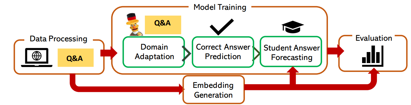
2. METHODOLOGY
The student answer forecasting pipeline depicted in Figure 1 is based on students interactions with MCQs in an ITS named Lernnavi. The pipeline predicts the likelihood of a student selecting a particular MCQ answer, based on the question and answer text and a student embeddings generated from their historical interaction data. In this section, we describe each step of the pipeline.
2.1 Data Processing
Learning Context. We focus our analyses on data collected from Lernnavi, an ITS for high-school students. Lernnavi offers adaptive learning and testing sessions in mathematics and language learning.
Dataset. The dataset is characterized by the following three data representations: 1) user-generated interactions, also referred to as “transactions“ (\(I_u^s = {i_1, \ldots , i_K}\) for each user \(u\)), 2) Lernnavi questions also referred to as “documents”, representing the associated questions (\(\mathbb {Q}^s\)), answer choices (\(\mathbb {C}^s\)), and textual pages provided to students, and 3) the taxonomy of topics (\(\mathbb {T}\)) shown in the German and Math dashboards. We only consider “documents” regarding German MCQs with at least one transaction from a user. After filtering, the dataset is composed of 237 unique questions and 138,149 transactions. Moreover, the dataset consists of 10,499 users with at least one transaction for German MCQs. The median number of MCQ answers from learners is 7 with some learners that answered up to 311 questions (including multiple trials for the same question).
2.2 Problem Formulation
We analyze users \(U^s \subset \mathbb {U}\) engaging in learning sessions \(s\) within Lernnavi’s \(\mathbb {S}\) offerings, focusing on sessions \(S = {s_1, \ldots , s_{M^S}}\), each a unique iteration within a broader topic \(t \subset \mathbb {T}\). These sessions are characterized by their interactive quizzes, sourced from a question bank \(\mathbb {Q}^s\) and designed to assess user knowledge through multiple-choice formats. Interactions in these sessions are represented as \(I_u^s = {i_1, \ldots , i_K}\) for each user \(u\), involve selections (\(c\)) from the provided answer options for each question \(q\).
These interactions are timestamped and detailed to capture the essence of user engagement and learning behavior. To evaluate user trajectories, we introduce binary metrics for answer choices, \(\mathbb {C}^s = {c_{q_1}, \ldots , c_{q_{|Q^s|}}}\), allowing for an in-depth analysis of user response selection. This design is to enable the multi-response setting for question \(q\), which can either have one correct answer choice \(c_{q_i}\) or multiple correct answer choices \(\mathbb {C}_{q}\), of which user \(u\) chooses one answer \(c_{q_u}\) or multiple \(\mathbb {C}_{q_u}\).
The answer-forecasting prediction task is to predict for a given user \(u\) with past interaction history \(I_u^s\), which answer choices \(\mathbb {C}_{q}\) are most likely to be chosen by the student.
2.3 Embedding Generation
To create student embeddings for a prediction model, we
explored four strategies to make a total of 22 different
embeddings: one using the MLP model, 16 using the LSTM
models, one using LernnaviBERT, and four using Mistral 7B
Instruct models:
MLP Autoencoder Embedding: We utilized a Multilayer
Perceptron (MLP) autoencoder with specific architecture and
feature engineering to encode students’ previous performance,
resulting in a size of 11907.
LSTM Autoencoder Embedding: We considered four stacked
LSTM configurations with varying sequence lengths and number
of layers to balance computational complexity and richness of
student interaction history.
LernnaviBERT Embedding: We created
embeddings using a finetuned German BERT base
model1to MCQ-specific language, LernnaviBERT, with a sequence
length of 10 and mean pooling strategy.
Mistral 7B Instruct Embedding: We used Mistral 7B Instruct
to generate embeddings with sequence lengths of 10, 20, 30, and
40 with mean pooling at the penultimate layer.
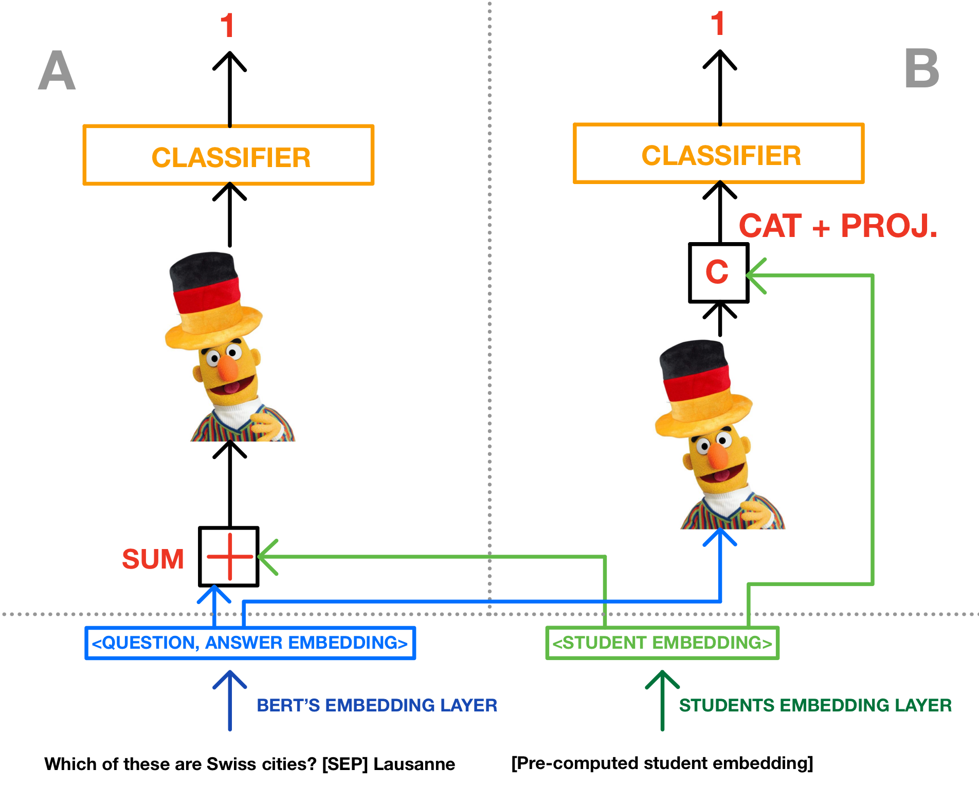
MCQStudentBertSum (A) and MCQStudentBertCat
(B) architectures.
In MCQStudentBertSum, the student embeddings are summed
with LernnaviBERT question embeddings at the input, before
being passed to the MCQBert model and classification layer.
In MCQStudentBertCat, MCQ embeddings are generated
with LernnaviBERT, then passed to the MCQBERT model
and concatenated with the student embeddings just before
the classification layer. German BERT image taken from
https://www.deepset.ai/german-bert
2.4 MCQStudentBert: Answer Forecasting
We initially train an MCQBert for the classification of
correct/incorrect MCQ answers. Learning the correct answers
across all MCQs is necessary to ensure that any failure in
predicting a student’s response did not arise from a lack of
knowledge of the correct answer. Appendix 5.1 details the
training and evaluation strategy.
We then extend MCQBert to include the students’ history
and predict students’ responses to MCQs. Inputs for this
task include the text of the MCQs and supplementary
student-specific data encapsulated within embeddings. The
objective has changed; rather than pinpointing the correct
answers from available options, the emphasis is on predicting
the actual responses provided by students. This task continues
to be treated as a binary classification problem. Details are
included in Appendix 5.2.
We explore the two models in Figure 2, differing in their handling
of student embeddings for integrating student information
into the prediction process: MCQStudentBertCat where the
inputs are concatenated before the classification layer and
MCQStudentBertSum2
where the embeddings are summed at the input. Both
models are based on MCQBert, finetuned in the previous
phase of the pipeline. These variants are augmented with a
classifier head, comprising two linear layers with a ReLU
activation function, to predict the likelihood of each potential
answer being chosen by a student. Inset B of Figure 2
illustrates MCQStudentBertCat strategy. The concatenation
strategy draws inspiration from context-aware embeddings
[27, 28], where additional features (like user or product
embeddings) are appended before the final classification layer
to provide context. For this purpose, in our context, the
student embeddings are first transformed using a linear layer
to match the MCQBert’s hidden size. These transformed
embeddings are then concatenated with the output of the
MCQBert model which is the representation of the first token
[CLS] token. This approach leaves the MCQBert processing
unchanged and appends additional information right before the
final decision-making process (e.g., classification). It allows
the classification model to consider both the processed
input representation and the student-specific information
distinctly.
In contrast, MCQStudentBertSum, depicted in Figure 2 (inset A),
integrates the student embeddings directly into the input
embeddings of the MCQBert model. This approach is similar to
multimodal learning for LLMs to create combined embeddings
that represent both modalities at the input level (e.g. to
create visual-semantic embeddings) [29]. Specifically, the
student embeddings are first transformed to match the
dimensionality of the MCQBert input embeddings using a
linear layer. These transformed student embeddings are
then summed with the original input embeddings. This
approach alters the initial representation that the MCQBert
model processes. The student embeddings can be seen as providing an initial bias or modification to the input
embeddings, potentially allowing the model to adapt more
specifically to characteristics represented by the student
embeddings.
3. EXPERIMENTAL EVALUATION
We finetune LernnaviBert to predict the correct MCQ answer,
resulting in MCQBert. Next, we integrate the student embeddings
(RQ1) to forecast student answers to produce variations of
MCQStudentBert (RQ2). The experimental evaluation of
MCQBert for correct answer prediction can be found in Section
5.1
We evaluate the different embedding strategies and ways of
integration to predict student responses to MCQ. A key
difference from MCQBert is the incorporation of student
embeddings, enabling models to use contextual information.
Embedding Performance. The training of the MLP autoencoder yielded a mean validation loss of \(1.3e^{-7}\). Further analysis highlighted a discrepancy in the norm-2 distance between the input and output vectors across training, validation, and test datasets, with an average input norm-2 (\(\lVert input \rVert _2\):) of 1.31 and an average discrepancy norm-2 (\(\lVert input - output \rVert _2\)) of 0.03. The LSTM models yielded a mean validation loss of \(1.3e^{-2}\) with a mean input norm of 13.59 and an average reconstruction norm of 10.94.
We did not find a trend in the number of hidden layers for the
LSTM. For subsequent analyses, the single-layer LSTMs are
used. After tuning, for both Mistral 7B and LSTMs, the best
sequence length was 20.
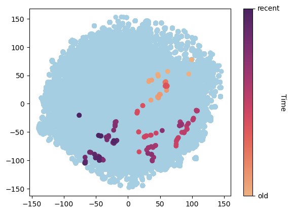
LernnaviBERTembedding
space. Highlighted is the evolution of a single student’s
embedding through time.
To examine the LernnaviBERT embeddings in detail, Figure 3
visualizes the embedding space using t-SNE. Each point
represents a student-embedding at a given time. Students are
represented by multiple points, reflecting the evolution of their
embeddings as they respond to successive MCQs. In Figure 3,
the trajectory of embeddings from an individual student is
accentuated. The temporal aspect of these embeddings is
depicted through a color gradient, transitioning from lighter
shades for initial interactions to darker shades for more recent
activity. The highlighted trajectory suggests a discernible shift
in the student’s embedding space over time from the upper right
to the lower left corner.
Predictive Model Performance. A total of 20 models were trained, incorporating 10 distinct embeddings and 2 integration strategies, over three epochs3. The models were evaluated on a hold-out test set consisting of MCQs previously encountered by the model, but not in the context of the specific student being assessed.
The optimal performance for all models was recorded in either
the second (followed by a marginal decline in the third
epoch) or third epoch. Table 1 presents the results from
the best epoch, showcasing both integration strategies
(concatenation and addition) across four embedding types
(MLP, LSTM, LernnaviBERT, Mistral 7B), compared to a
baseline Dummy Classifier and MCQBert (no embedding). For
brevity, only the results from the best-performing LSTM,
with 1 hidden layer and a sequence length of 20, and the
highest-achieving Mistral 7B model, with a sequence length of
20, are displayed3.
Integration Strategies. As seen in Table 1, the concatenation
strategy (MCQStudentBertCat) generally yields slightly better
results compared to the summation strategy (MCQStudent
BertSum), particularly noticeable with LernnaviBERT.
Embeddings. All embedding strategies show substantial
improvements over the Dummy Classifier across all metrics.
Mistral 7B is the best-performing embedding for both
integration strategies (MCQStudentBertCat, MCQStudentBertSum).
When applied to MCQStudentBertCat, the Mistral 7B
embedding shows a notable increase in performance metrics: an
improvement of 0.579 in MCC, 0.477 in F1 score, and 0.207 in
accuracy compared to the Dummy Classifier. For the second
baseline (MCQBert), the Mistral 7B embedding showed a 12%
improvement.
Consistency is observed in the performance ranking of
embeddings between the two integration strategies. In the
MCQStudentBertCat configuration, LernnaviBERT ranks second
with an \(MCC=0.575\), followed by the LSTM autoencoder with \(MCC=0.567\), and
the MLP autoencoder trailing with \(MCC=0.557\). Similarly, for the
MCQStudentBertSum strategy, the LernnaviBERT embedding is in
the second position \(MCC=0.575\) followed by the LSTM autoencoder with an
\(MCC=0.564\), while the MLP autoencoder remains the least effective, with
an \(MCC=0.552\).
The performance differentials between embeddings are marginal.
For instance, within the MCQStudentBertCat framework Mistral
7B, exhibits a modest 4% improvement in MCC over the MLP
autoencoder. Similarly, in the MCQStudentBertSum framework,
the margin is 3%.
4. DISCUSSION AND CONCLUSION
Our goal is to enhance the predictive capabilities of ITS by developing embeddings that capture student interactions (RQ1) and integrating them into an answer forecasting model (RQ2) to improve performance and personalization.
We explored various methods of encoding students’ interactions
with the ITS including using autoencoders with MLP and
LSTM architectures, and LLMs including LernnaviBERT model
and Mistral 7B (RQ1). Our findings revealed that the Mistral
7B embedding emerged as the best-performing method for our
use-case, demonstrating a 12% performance enhancement
relative to MQCBert (baseline with no embedding) and a 4%
improvement over the least effective embedding, the MLP
autoencoder. The performance of Mistral 7B, closely followed
by LernnaviBERT, LSTM, and MLP autoencoder can be likely
attributed to the inherent capabilities of each embedding
approach in capturing and representing student interactions.
For example, Mistral 7B has a sliding window attention
mechanism, facilitating a deeper understanding of contextual
relationships within student data [30]. This model’s efficacy
is further augmented by its fine-tuning on instructional
datasets, potentially enhancing its proficiency in interpreting
question-answer pairs. Moreover, LernnaviBERT also seemed to
capture the contextual information of educational interactions
effectively, ranking it closely behind Mistral 7B. The slight
difference in performance between these two models may be due
to Mistral 7B’s more advanced mechanisms for handling long
sequences and its ability to incorporate broader contextual
information. Notably, the optimal sequence length for Mistral
7B was identified as 20, whereas the LernnaviBERT model was
constrained to sequence lengths of 10 due to its context
limitations. This is further supported by the Mistral 7B
embedding visualizations that show a more discernible trend
with sequence lengths greater than 10. The LSTM autoencoder
underperforms compared to transformer-based models
because it prioritizes temporal dynamics over deep contextual
understanding. While its sequential processing is good for
capturing learning progression, it may not handle complex
language structures as well as transformer models. The
low performance scores of the MLP autoencoder can be
attributed to its simpler architecture, which may not capture
complex language-based information and temporal dynamics
effectively.
To study the integration of student interaction embeddings
into an answer forecasting model (RQ2), we used two
approaches: MCQStudentBertCat, which concatenates student
embeddings with model outputs before classification, and
MCQStudentBertSum, which sums the embeddings at the input
stage. The superior performance of the MCQStudentBertCat
model compared to the MCQStudentBertSum model could be
attributed to its ability to maintain a clear separation between
the question-answer information and the student-specific
embeddings, promoting distinct utilization of both sources of
information in the prediction process. Future research could
further explore the optimization of such integration techniques,
potentially investigating the impact of varying the point of
concatenation.
One limitation of our study is the interpretability of the
embeddings generated by the models we explored, such as
LernnaviBERT and Mistral 7B. Despite their effectiveness, there
is a significant gap in our understanding of the underlying
features and feature patterns encapsulated by these embeddings,
hindering our ability to comprehend their effectiveness. The
generalizability of our findings is limited by the study’s
execution within a single context and the lack of publicly
available datasets comparable in richness to Lernnavi. However,
our study aligns with and contributes to the growing body of
research in answer forecasting by incorporating student history
into predictive models. We aim to introduce a novel approach
that can be replicated by the EDM community in different
ITS and contexts, enabling a better understanding of the
generalizability of our findings and fostering advancements in
personalized instruction.
In conclusion, we introduce MCQStudentBert, a model for
student answer forecasting that leverages LLMs to integrate the
contextual understanding of question and answer texts with
students’ historical interactions. Our work contributes to the
field of EDM in the German language context, where such
studies are scarce, and promotes the use of open-source models,
facilitating wider adoption and adaptation within the EDM
community. Furthermore, our model’s utility extends to ITS,
where it can be employed to tailor potential answers for
individual learners and give hints dynamically. From the
educator’s and developers’ perspective, it is possible to modify
or augment the answer choices without necessitating a complete
retraining of the model. This feature could allow seamless
updates and expansions to the answer sets in response
to evolving pedagogical requirements or teacher/student
feedback.
Acknowledgements. This project was substantially funded by the Swiss State Secretariat for Education, Research and Innovation (SERI) and the Swiss Canton of St. Gallen.
References
- Neil T Heffernan and Cristina Lindquist Heffernan. The assistments ecosystem: Building a platform that brings scientists and teachers together for minimally invasive research on human learning and teaching. International Journal of Artificial Intelligence in Education, 24:470–497, 2014.
- Ghodai Abdelrahman, Qing Wang, and Bernardo Nunes. Knowledge tracing: A survey. ACM Computing Surveys, 55(11):1–37, 2023.
- Tanja Käser, Gian-Marco Baschera, Juliane Kohn, Karin Kucian, Verena Richtmann, Ursina Grond, Markus Gross, and Michael von Aster. Design and evaluation of the computer-based training program calcularis for enhancing numerical cognition. Frontiers in psychology, 4:489, 2013.
- John R Anderson, Albert T Corbett, Kenneth R Koedinger, and Ray Pelletier. Cognitive tutors: Lessons learned. The journal of the learning sciences, 4(2):167–207, 1995.
- Tirth Shah, Lukas Olson, Aditya Sharma, and Nirmal Patel. Explainable knowledge tracing models for big data: Is ensembling an answer? arXiv preprint arXiv:2011.05285, 2020.
- Albert T Corbett and John R Anderson. Knowledge tracing: Modeling the acquisition of procedural knowledge. User modeling and user-adapted interaction, 4:253–278, 1994.
- Chris Piech, Jonathan Bassen, Jonathan Huang, Surya Ganguli, Mehran Sahami, Leonidas J Guibas, and Jascha Sohl-Dickstein. Deep knowledge tracing. Advances in neural information processing systems, 28, 2015.
- Hiromi Nakagawa, Yusuke Iwasawa, and Yutaka Matsuo. Graph-based knowledge tracing: modeling student proficiency using graph neural network. In IEEE/WIC/ACM International Conference on Web Intelligence, pages 156–163, 2019.
- Sami Sarsa, Juho Leinonen, and Arto Hellas. Empirical Evaluation of Deep Learning Models for Knowledge Tracing: Of Hyperparameters and Metrics on Performance and Replicability. Journal of Educational Data Mining, 14(2), 2022.
- Hao Cen, Kenneth Koedinger, and Brian Junker. Learning factors analysis–a general method for cognitive model evaluation and improvement. In International conference on intelligent tutoring systems, pages 164–175. Springer, 2006.
- Philip I Pavlik Jr, Hao Cen, and Kenneth R Koedinger. Performance factors analysis–a new alternative to knowledge tracing. Online Submission, 2009.
- Alisa Lincke, Marc Jansen, Marcelo Milrad, and Elias Berge. The performance of some machine learning approaches and a rich context model in student answer prediction. Research and Practice in Technology Enhanced Learning, 16(1):1–16, 2021.
- Zichao Wang, Angus Lamb, Evgeny Saveliev, Pashmina Cameron, Yordan Zaykov, José Miguel Hernández-Lobato, Richard E Turner, Richard G Baraniuk, Craig Barton, Simon Peyton Jones, Simon Woodhead, and Cheng Zhang. Diagnostic questions: The neurips 2020 education challenge. arXiv preprint arXiv:2007.12061, 2020.
- Shen Shuanghong, Liu Qi, Chen Enhong, Tong Shiwei, Huang Zhengya, Tong Wei, Su Yu, and Wang Shijin. Which to choose? an order-aware cognitive diagnosis model for predicting the multiple-choice answer of students.
- Si Chenglei, Wang Shuohang, Kan Min-Yen, and Jiang Jing. What does bert learn from multiple-choice reading comprehension datasets? 2019.
- Wang Zichao, Lamb Angus, Saveliev Evgeny, Cameron Pashmina, Zaykov Yordan, Hernández-Lobato José Miguel, Turner Richard E., Baraniuk Richard G., Barton Craig, Peyton Jones Simon, Woodhead Simon, and Zhang Cheng. Results and insights from diagnostic questions: The neurips 2020 education challenge. Proceedings of Machine Learning Research, (133):191–205, 2021.
- Yuto Shinahara and Daichi Takehara. Quality assessment of diagnostic questions based on multiple features, 2020.
- Zhang Hongbo, Qin Xiaolei, Zou Wuhe, Zhu Yue, Liu Ying, Liang Nan, and Zhang Weidong. How to predict students’ interactions with diagnostic questions: from a perspective of recommender system.
- Aritra Ghosh and Andrew S Lan. Option tracing: Beyond binary knowledge tracing.
- Benoît Choffin, Fabrice Popineau, Yolaine Bourda, and Jill-Jênn Vie. Das3h: modeling student learning and forgetting for optimally scheduling distributed practice of skills. arXiv preprint arXiv:1905.06873, 2019.
- Ahatsham Hayat and Mohammad Rashedul Hasan. Personalization and Contextualization of Large Language Models For Improving Early Forecasting of Student Performance. In NeurIPS Workshop on Generative AI for Education (GAIED), 2023.
- Xu Guowei, Chen Jiaohao, Li Hang, Kang Yu, Liu Tianqiao, Hao Yang, Ding Wenbiao, and Liu Zitao. Solution for neurips education challenge 2020 from tal ml team.
- Manh Hung Nguyen, Sebastian Tschiatschek, and Adish Singla. Large Language Models for In-Context Student Modeling: Synthesizing Student’s Behavior in Visual Programming from One-Shot Observation. ArXiv, abs/2310.10690, 2023.
- Shishir Roy, Nayeem Ehtesham, Md. Saiful Islam, and Marium-E-Jannat. Augmenting bert with cnn for multiple choice question answering. In 2021 24th International Conference on Computer and Information Technology (ICCIT), pages 1–5, 2021.
- Joshua Robinson, Christopher Michael Rytting, and David Wingate. Leveraging large language models for multiple choice question answering. arXiv preprint arXiv:2210.12353, 2022.
- Thiemo Wambsganss, Vinitra Swamy, Roman Rietsche, and Tanja Käser. Bias at a second glance: A deep dive into bias for german educational peer-review data modeling. COLING, 2022.
- Xinlong Li, Xingyu Fu, Guangluan Xu, Yang Yang, Jiuniu Wang, Li Jin, Qing Liu, and Tianyuan Xiang. Enhancing bert representation with context-aware embedding for aspect-based sentiment analysis. IEEE Access, 8:46868–46876, 2020.
- Ashish Vaswani, Noam Shazeer, Niki Parmar, Jakob Uszkoreit, Llion Jones, Aidan N. Gomez, Lukasz Kaiser, and Illia Polosukhin. Attention is all you need, 2023.
- Jiacheng Chen, Hexiang Hu, Hao Wu, Yuning Jiang, and Changhu Wang. Learning the best pooling strategy for visual semantic embedding. In Proceedings of the IEEE/CVF conference on computer vision and pattern recognition, pages 15789–15798, 2021.
- Albert Q Jiang, Alexandre Sablayrolles, Arthur Mensch, Chris Bamford, Devendra Singh Chaplot, Diego de las Casas, Florian Bressand, Gianna Lengyel, Guillaume Lample, Lucile Saulnier, et al. Mistral 7b. arXiv preprint arXiv:2310.06825, 2023.
5. APPENDIX
This appendix includes additional figures and material to complement the main section of the paper.
| MCC | F1 Score | Accuracy | |
|---|---|---|---|
| Dummy Classifier | 0 | 0.292 | 0.605 |
MCQBert | 0.472 | 0.702 | 0.740 |
![At the top, a binary classifier receives input from the [CLS] token of a BERT model. The BERT model processes input sequences including a classification token [CLS], question tokens, a separator token [SEP], and answer tokens. The BERT model consists of a transformer encoder, depicted as layers of multi-head attention and feed-forward neural networks with positional encoding. An inset on the right illustrates the internal structure of the transformer encoder.](./figures_3_report.png)
MCQBERT Architecture. The MCQBERT model for
correct answer prediction involves a binary classifier and a
finetuned BERT architecture predicting answers in sequence.
The inset showing the Transformer encoder is taken from [28].

Mistral
   7B
embedding space for difference sequence lengths. The evolution of the same
student’s embedding through time is highlighted.
5.1 MCQBert: Correct Answer Prediction
This section introduces MCQBert, a model developed to
predict students’ responses to MCQs using only the question
text4.
The downstream task and primary objective of MCQBert is to
accurately identify the correct answer(s) from the given
options in each MCQ in the dataset. The architectural design
of MCQBert is illustrated in Figure 6. It represents the
LernnaviBERT model’s application in processing both the
question and a potential answer as input sequences. The
transformer encoder component of LernnaviBERT processes the
sequences before it is passed to a binary classifier, which
outputs ‘1’ for a correct answer and ‘0’ for an incorrect
one.
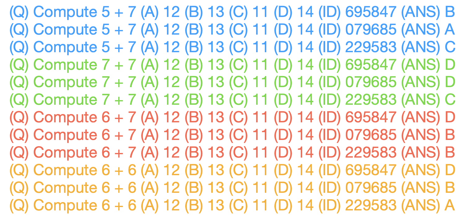
Data Split. To formulate the MCQ prediction challenge as a binary classification task, each MCQ datapoint is decomposed into separate instances, each pairing the question with a possible answer option. The model thus aims to assign a ‘1’ to a correct or student-selected answer and a ‘0’ to an incorrect or unselected answer.
We implement a partitioning ratio of 80/10/10 for training, validation, and testing, respectively. Notably, each MCQ occurs multiple times within the dataset, corresponding to different answers. To rigorously assess the model’s ability to generalize and accurately answer new MCQs, we ensure that individual MCQs are exclusively allocated to either the training or the testing set. In other words, all occurrences of a particular MCQ are confined to a single subset.
Experiments. To evaluate the performance of our models in predicting correct answers to MCQs, two distinct experiments were conducted. In the first one, the model was fine-tuned using the designated training set, and its generalization capacity was assessed on a separate test set comprising unseen questions, validating its ability to respond to MCQs beyond the training data. The second experiment involved training the model on the entire MCQ dataset, confirming its effective learning of correct answers across all MCQs, ensuring that any failure in predicting a student’s response did not arise from a lack of knowledge of the correct answer. In the final phase of our pipeline for predicting student responses to MCQs, the model trained on the complete dataset was fine-tuned, allowing it to utilize its comprehensive knowledge of the correct answers when making predictions.
This section describes the evaluation of MCQBert’s performance
in the specific task of predicting correct answers to MCQs. The
evaluation consisted of two distinct experiments, each employing
a different training procedure to assess the model’s predictive
capabilities.
Experiment 1: Model Evaluation Against Unseen MCQs. The first experiment aimed to evaluate the ability of the model to predict the correct answers of previously unseen MCQs accurately. The models were fine-tuned for one epoch on a designated training set and subsequently evaluated on a separate test set. The evaluation metrics included MCC, F1 score, and accuracy.
The results, as summarized in Table 2, contrast the performance
of MCQBert with that of a Dummy Classifier, a baseline always
predicting the majority class (i.e. 0). This comparison is useful
for evaluating the effectiveness of MCQBert beyond simple chance
or biased class distribution.
The performance metrics indicate that MCQBert outperforms the
baseline Dummy Classifier, evidencing its capability to discern
correct answers in the context of MCQs.
Experiment 2: Model MCQs Retention Evaluation. The second
experiment was designed to evaluate MCQBert’s capacity for
retaining correct answers after being fine-tuned on the entire
Lernnavi MCQ dataset. The model was then tested on
the same dataset to assess its ability to recall the correct
answers, effectively evaluating its memorization capability. Not
surprisingly, MCQBert achieved an MCC of 0.983, indicating
nearly perfect recall of the correct answers within the dataset.
This high level of performance is further corroborated by F1
scores of 0.993 for class 0 and 0.989 for class 1. The accuracy
score of 0.992 reinforces the model’s strong predictive capability
and suggests that MCQBert model has learnt the correct answers
to the vast majority of the MCQs present in the dataset,
and we can therefore exploit this knowledge in the next
step.
5.2 Reproducibility for MCQStudentBERT
Similar to the MCQ prediction task without student data, we
split the dataset into training, validation, and test datasets
using an 80/10/10 split. In contrast to the base model
(MCQBert), where each question-answer pair was exclusively
assigned to one subset, in this task, individual MCQs can be
present in both training and testing phases due to multiple
representations within the dataset. This decision allows the
model to leverage prior history related to specific questions,
enhancing predictive accuracy by considering responses from
students who share similar characteristics with the target
student.
Evaluation Metrics. We assess our models using three different metrics: the Matthews Correlation Coefficient (MCC) for binary classification, the F1 score for balancing precision and recall, and the accuracy score for overall predictions. MCC and F1-score are effective even if the classes are strongly imbalanced, motivating our evaluation choices. While accuracy and F1-score range between 0 to 1, MCC is a correlation coefficient value between -1 and +1 (+1: perfect prediction, 0: average random prediction, -1: inverse prediction).
5.3 Impact of sequence length on latent space representations
We examined the sequence length impact on the Mistral 7B
embeddings. Similar to Figure 3, Figure 7 shows a single
student’s embeddings across varying sequence lengths. Echoing
the behavior of the LernnaviBERT embedding, we note a
discernible diagonal progression in the embeddings when the
sequence length is greater than 10. The trend suggests that as
the sequence length increases, the student’s representation in
the embedding space demonstrates a more pronounced
diagonal trajectory, transitioning methodically from older to
more recent embeddings with a progressively smoother
evolution.
1https://huggingface.co/google-bert/bert-base-german-cased
2MCQStudentBertCat and MCQStudentBertSum are available at https://go.epfl.ch/hf-answer-forecasting
3Full results are available at https://go.epfl.ch/mcq-results
4MCQBert is available at
https://huggingface.co/collections/epfl-ml4ed/student-answer-forecasting-edm-2024-663b7c20bb2aa3273dda4de2