ABSTRACT
GRE Aptitude Test scores have been a key criterion for admissions to U.S. graduate programs. However, many universities lifted their standardized testing requirements during the COVID-19 pandemic, and many decided not to reinstate them once the pandemic ended. This change poses additional challenges in evaluating prospective students. In this paper, we examine the viability of applying machine learning models to predict applicant GRE scores using their application materials. We utilize a diverse set of information from the admissions application, including undergraduate GPA, undergraduate major, and resume. This study is based on 814 MS in Computer Science and M.S. in Data Science applications, each submitted with GRE scores. The induced prediction models can serve as a focus of attention (FOA) tool for admissions committees and aid in rendering scholarship and rejection decisions. We further identify and discuss the principal factors utilized by our models to better understand the relationship between the various application components and GRE performance. Our findings also suggest the factors that one might focus on when GRE scores are unavailable.
Keywords
1. INTRODUCTION
The Graduate Record Examination (GRE) is a cognitive abilities test administered by Educational Testing Service (ETS). The test consists of three components that measure applicants’ competence in verbal reasoning (GRE-V), quantitative reasoning (GRE-Q), and analytical writing skills (GRE-A). Because of its objectivity, standardization, and predictive utility, GRE scores are used by many graduate schools as necessary criteria to admit qualified students. Indeed, an earlier study led by Norcross et al. showed that more than 90% of Ph.D. programs and over 80% of master’s programs in the U.S. mandated GRE scores [20]. Despite GRE’s essential role in graduate admissions, many institutions were forced to lift the requirement due to the COVID-19 pandemic. The main concerns are the accessibility to physical test centers and potentially compromised scores from at-home tests. As a result, admission committees have to rely on more subjective materials such as the statement of intent (SOI) and letters of recommendation (LORs). Adequate estimation of missing GRE scores is valuable in two respects. First, it will facilitate an equal evaluation of all applicants in the absence of standardized test scores. Second, for programs that currently mandate GRE scores, reliable predictive models can help to eliminate the GRE requirement and make the GRE exam optional or encouraged. Such a change can lead to a more diverse pool of students and accommodate disadvantaged students from rural and low-income backgrounds [12].
| Demographics | TOEFL Scores | CS Skills* |
|---|---|---|
| Gender | Listening | Python |
| Race | Speaking | Java |
| Age | Reading | C++ |
| Permanent Country | Writing | Matlab |
| Native English Speaker | SAS | |
| Math Skills* | Database | |
| Academic Credentials | Calculus | Microsoft Office |
| Undergraduate Major | Linear Algebra | Machine Learning |
| Undergraduate GPA | Statistics | Software |
| Months Since Degree |
* Binary features indicating if the applicant’s resume contains the keyword.
This study investigates the viability of predicting missing applicant GRE scores using the rest of their application materials. The underlying assumption is that students’ academic credentials and professional experiences are highly correlated to their performance on standardized tests. For example, applicants who have taken math courses (e.g., linear algebra or statistics) are likely to perform well in the quantitative section of the GRE test, and students’ GPAs could be positively correlated with their GRE scores. We utilized information extracted from student application materials and grouped it into five categories: demographics, academic credentials, TOEFL performance (for international students), Math skills, and Computer Science (CS) skills. Table 1 presents the predictors utilized for this study. These features are extracted from student application materials and grouped into five categories: demographics, academic credentials, TOEFL performance (for international students), Math skills, and Computer Science (CS) skills. We present the engineering of these features and their statistics in Section 3.
We build our predictive models using over 800 applications that include GRE scores from two graduate programs at Fordham University. We also explore machine learning approaches for two GRE prediction tasks. First, we employ regression models to predict GRE-Q and GRE-V score percentiles. Percentiles are employed rather than raw scores as they are more easily interpreted. The evolution of GRE scoring also influenced this choice, as the GRE scoring scales have changed over time, while the percentiles remain consistent across these changes. In the second task, we build classification models to identify the top 20% and bottom 20% of applicants, respectively, based on their GRE-Q or GRE-V scores. Given that the learned classification models help identify top and bottom applicants in the pool, they can serve as a Focus of Attention (FOA) tool to facilitate scholarship and rejection decisions. The undertaking of the second task is particularly valuable in reducing the workload of the admission committees given the continuous rise in graduate applications [10]. Our study further examines separate models for international students, which leverages their standard foreign language test scores (e.g., TOEFL), which have been shown to be correlated with GRE performance[1].
We further investigate the principal factors in estimating applicant GRE scores. The identified top predictors can be used for two purposes. First, they pinpoint the application components that are most relevant to the applicants’ GRE abilities and, thus, can facilitate efficient and systematic applicant comparisons in the absence of GRE scores. Second, the principal predictors can help us identify and analyze potential racial and gender biases associated with GRE scores. A prior study has found that “the GRE is a better indicator of sex and skin color than of ability and ultimate success” [16]. Our study, however, suggests that gender and race are not top predictors for GRE scores. We present and discuss our principal predictors in Section 5.4.
2. RELATED WORK
Investigating the validity of the GRE test and its predictive value in student performance in higher education is an active research area. Kuncel et al. launched extensive research examining the effectiveness of GRE in predicting performance at both the master’s and doctoral levels. They found that GRE scores, over nearly 100 studies and 10,000 students, predict first-year and overall GPAs well for both master’s and doctoral students [13]. Young et al. investigated the validity of the GRE scores in the admission of Master of Business Administration (MBA) students using a sample of 480 admitted students[29]. They found that for predicting student first-term GPAs, GRE-Q was the most influential predictor, followed by GRE-V and GRE-A. Furthermore, they found that the three GRE test metrics are significantly more predictive than undergraduate GPAs.
Despite the value of standardized testing, some studies have found the evidence supporting the use of GRE scores to be controversial and therefore advocate for the elimination of the GRE test. For example, Petersen et al. presented a multi-institutional study of GRE scores as predictors of STEM Ph.D. degree completion [21]. Their findings suggest that GRE scores are not a strong predictor of graduate school success and, thus, should not be considered the gold standard for admission. Likewise, Sealy et al. investigated the association between GRE scores and academic success among Ph.D. students in biomedical sciences [22]. They concluded that the GRE scores were weak predictors of future academic success. In addition to questioning the predictive value of the GRE scores, researchers have also raised concerns about the test’s fairness and implicit bias, considering the wide achievement gap in test scores between demographic groups [12, 18, 27].
All of the above studies focused on evaluating the validity of the GRE. Our study differs in that we investigate the possibility of predicting applicant GRE performance using readily available application materials, and in understanding which application materials are most closely associated with the GRE scores. However, some prior work has investigated the relationship between some of the information provided in a graduate application and GRE scores. One study of a Masters program in engineering showed statistically significant correlations between TOEFL scores and GRE Verbal (r=.63), GRE Quantitative (r=.30), and GRE Analytical (r=.35) scores [1], while another study showed a positive correlation between undergraduate GPA and GRE scores [19].
Other studies have shown significant connections between demographic categories and GRE scores. One study that examined GRE scores from 1982 to 2007, when GRE scores ranged from 200-800, observed that men performed, depending on the year, between 20 and 34 points higher than women on GRE verbal scores and 76 to 84 points better on the quantitative scores [3]. A more recent study [8] covering the period 2022-2023 showed that men outperformed women by 1 point on the GRE verbal score and by 4.5 points on the GRE quantitative score, using the newer GRE scale that ranges from 130-170. Additionally, a study of GRE scores in 1981 through 1982 found that GRE quantitative scores for international students are comparable to those for students from the United States, but the U.S. students have higher verbal and analytical GRE scores [26]. The same study showed that on the verbal scores, foreign students that come from countries where English is the primary language outperform their counterparts where English is not the primary language, but also still lag the students from the United States. A more recent study by the Educational Testing Service of GRE scores from 2015-2020 shows that U.S. citizens outperform non-U.S. citizens on verbal scores (151.8 to 151) but substantially underperform non-U.S. citizen on quantitative scores (150.5 to 161.5) [8].
3. DATA AND PRE-PROCESSING
Our study is based on 814 GRE-available applications submitted to the MS of Data Science (MSDS) and MS of Computer Science (MSCS) programs at Fordham University. Of these, 300 are international applications. The features we collected from the applications include demographics, academic credentials, and TOEFL scores for international students. We also programmatically extracted the skills from applicant resumes and generated binary features to indicate the presence of math and programming skills that are highly relevant to STEM programs. Table 1 presents the features used in this study.
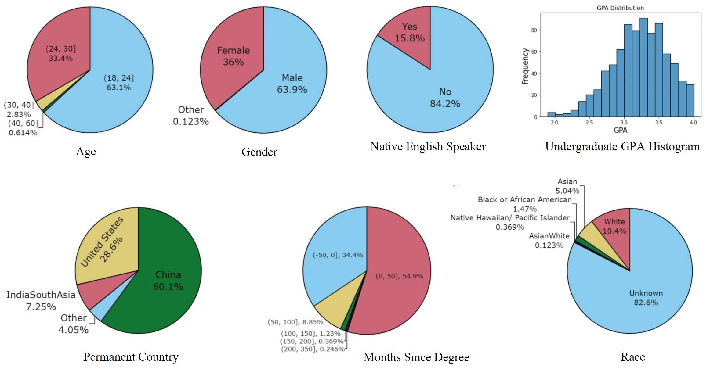
Approximately 96% of the applicants in our dataset are under age 30, with two-thirds of these under age 24. Slightly more than one-third (36%) of the applicants are female, which is consistent with the Computer Science and Data Science fields in the United States being male-dominated. Indeed, our applicant pool has more gender diversity than an average STEM program based on the U.S. Bureau of Labor Statistics for 2021 [25], which shows that women staff only 26% of the Computer and Mathematical occupations in the U.S. In addition, 84% of the applicants did not list English as their first language, which is partially due to a large number of international applicants. Our study does not consider racial information because it is optional in the application and 82% of the applicants did not provide it.
As mentioned earlier, the full list of features utilized by the prediction models are provided in Table 1. The features in the “Math Skills” and “CS Skills” categories are all binary features indicating whether the applicant’s resume contains the matching keyword (e.g., the “C++” feature is set to 1 if the resume contains “C++”).
These resume features are unverified by the university and may contain false information, which could impact the reliability of the learned models. However, this issue is not unique to the predictive approach, as such information can also influence human-made decisions. While it is conceivable that applicants, if privy to the model’s internals, might manipulate their resumes to increase their chances of admission, we consider this scenario to be highly unlikely, as institutions typically would not publicly disclose these models. Nonetheless, it’s important to recognize the potential consequences of utilizing unverified information, which is an area that warrants further investigation.
3.1 Feature Statistics
The distribution of key demographic and non-demographic feature values are summarized in Figure 1. The chart for age shows that the vast majority (96%) of applicants are under 30, with approximately two-thirds of these under 24 and the remaining one-third between 24 and 30. Only slightly more than one-third (36%) of the applicants are female, which is consistent with the Computer Science and Data Science fields in the United States being male-dominated. In fact, the applicant pool has more gender diversity than one might expect based on U.S. Bureau of Labor Statistics for 2021 [25], which show that only 26% of the Computer and Mathematical Occupations in the U.S. are staffed by women.
Figure 1 further shows that 84% of the applicants do not have English as their first language, which is mainly due to the large number of applicants from China and, to a lesser degree, India. In fact, 67% of applicants have China or India listed as their permanent country, although we know that even more come from these countries since many subsequently become US citizens (i.e., many of the 26% that list the US as their permanent country were born overseas). The racial information provided by the applicants is not very helpful since in 82% of the cases it is not specified. The Months since Degree information indicates the time from completion of the student’s last degree to the time of submitting the application. For 34% of the students this time is negative, indicating that they are applying while still completing their undergraduate degree, while most of the rest (55%) have completed their last degree within roughly the last four years. In less than 10% of the cases has the student completed their last degree more than four years ago.
We anticipated that the applicant’s prior grade point average (GPA) would be one of the key features for predicting the GRE scores, so it is important to have a good understanding of the GPA distribution. We expect most of the applicants to have good grades since the university’s policy is to only admit students with an undergraduate GPA of 3.0 or better. The GPA distribution of the applicants generally conforms to this, although 28% have a GPA below 3.0 and 5% a GPA below 2.5.
3.2 Applicant Prior Major Discipline
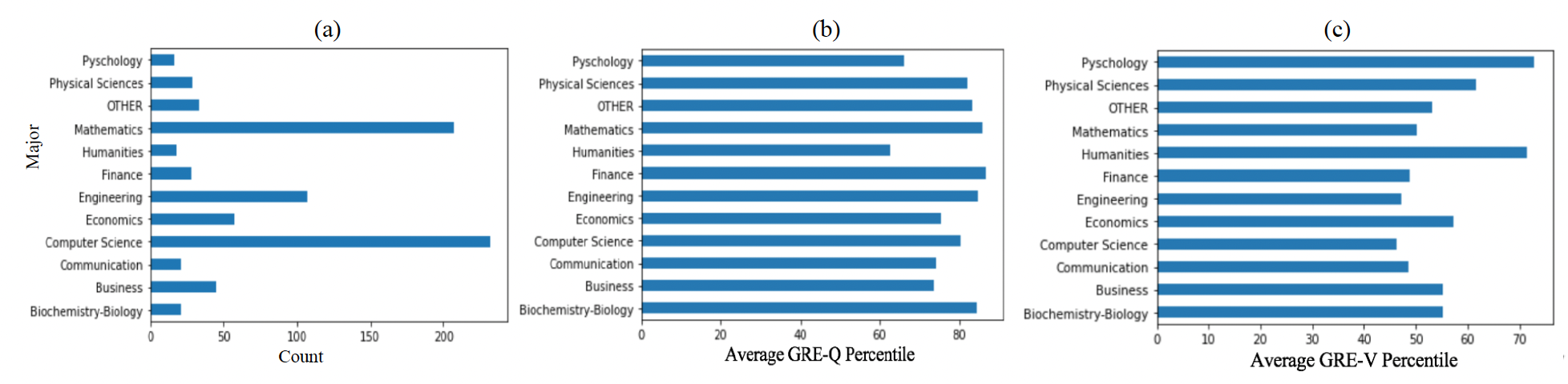
The applicant’s academic major is a particularly important feature since it provides a great deal of information about what prior education the student received. Figure 2(a) shows the distribution of the applicants by undergraduate major category. Because the MSCS and MSDS degrees are quite technical, one would expect most of the undergraduate degrees to be from STEM (Science, Technology, Engineering, and Math) fields, and that many would specifically be in Computer Science, since applicants to an MSCS program should generally have a Computer Science degree. The values in Figure 2(a) generally adhere to this, but there are a modest number of non-STEM (e.g., humanities, communication, economics, business) applicants.
One might expect the applicants with non-STEM degrees to have, on average, lower GRE quantitative scores and perhaps higher GRE verbal scores. This is largely what is observed in Figure 2(b) and Figure 2(c). Humanities majors have the lowest GRE-Q score, followed by psychology majors, and then economics, communications, and business majors. The psychology quantitative scores may seem anomalous, but psychology is sometimes considered a social science. Conversely, the STEM disciplines are associated with consistently high GRE-Q scores. Overall, the biggest surprise may be the very high GRE-Q scores for Finance majors. The patterns with the GRE-V scores tend to show that STEM majors yield low GRE-V scores and non-STEM fields yield higher GRE-V scores, but in many cases the fields perform similarly. The standouts are that psychology, humanities, and to a lesser degree economics, yield the highest GRE-V scores. Perhaps most surprising is that the communications majors have relatively low GRE-V scores.
3.3 GRE Score Percentile Distribution
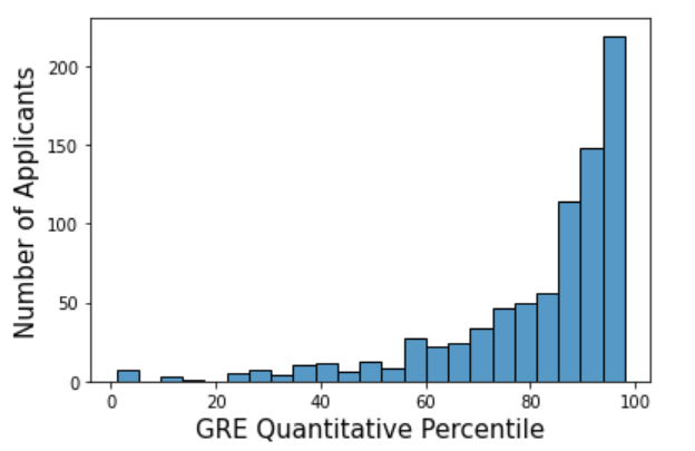
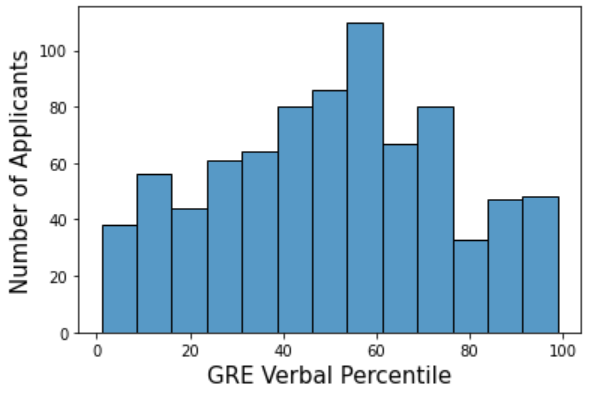
The distribution of the class variable is of special importance, and for that reason, we present in Figure 3 the percentile distributions of the GRE quantitative and verbal scores. The GRE-Q applicant percentile scores are heavily asymmetric and skewed toward the 100% percentile. This outcome is expected since applicants to the MSCS and MSDS degrees should have very high GRE-Q scores. It is worth noting, however, that while low scores are rare, they do exist (8% of applicants are below the 50th percentile), and extend all the way down to the very bottom. The distribution of GRE-V scores is much more symmetric and evenly distributed than the GRE-Q scores. Note that these different distributions have implications for the associated regression and classification tasks. Guessing the average value will yield much better regression results for the quantitative scores than the verbal scores since the quantitative scores are much more tightly concentrated. On the other hand, the nature of the problem will make it much harder to beat the strategy of always guessing the average value. Similarly, identifying the top 20% of GRE-Q percentile scores will not be easy since so many applicants have scores close to this border, but identifying the bottom 20% will not have this issue and therefore may be more achievable.
4. METHODOLOGY
This section briefly describes the models used for our regression and classification tasks, as well as the hyperparameter values used to train the models. These values were selected via grid search [6] using a nested 10-fold cross-validation on the training data. The unspecified hyperparameters were defaulted to the values in Python’s \(scikit\)-\(learn\) library, the software used to build our models. Next, we describe how we address the imbalanced training data. Lastly, we illustrate our model training and evaluation framework. This study was approved by the university’s Institutional Review Board, and informed consent was waived.
4.1 Regression Models
We experimented with three linear regression models in predicting the GRE-Q and GRE-V percentiles. These models applied different regularization techniques to prevent overfitting.
4.1.1 LASSO Regression
LASSO (Least Absolute Shrinkage and Selection Operator) regression [24] encourages simple, sparse models by adding the \(L_1\)-norm of model complexity to the cost function. In our study, we applied grid search to optimize the trade-off hyperparameter \(\lambda \). Depending on the specific tasks, the optimal \(\lambda \) values varied from 0.12 to 0.4.
4.1.2 Ridge Regression
Ridge regression [11] follows the same principle as LASSO except that it replaces the \(L_1\)-norm with the differentiable \(L_2\)-norm Ridge regression is desirable because the quadratic penalty term makes the cost function strongly convex, engendering a unique minimum and a closed-form solution. We further explored kernelized ridge regression with polynomial and RBF kernels. The best model was achieved using the RBF kernel with gamma = 0.01 and polynomial kernels with degrees ranging from 2 to 7.
4.1.3 Elastic Net
Elastic Net combines LASSO and ridge regression to exploit the advantages of both approaches. In addition, the elastic net encourages a grouping effect, where strongly correlated predictors tend to be in or out of the model together. The cost function of elastic net is defined as \[E(\mathbf {w}) = \frac {1}{N}\sum _{n=1}^{N}(\mathbf {w}^T\mathbf {x}_n-y_n)^2 + \lambda (\frac {(1-\alpha )}{2}||\mathbf {w}||_2 + \alpha ||\mathbf {w}||_1 \] where \(\alpha \) controls the trade-off between \(L_1\) and \(L_2\) regularization, and \(\alpha =1\) is equivalent to LASSO, and \(\alpha =0\) is equivalent to Ridge. Through grid search, we found that the optimal \(\lambda \) ranged from 0.06 to 0.38 for our models, and \(\alpha \) ranged from 0.7 to 1.
4.2 Classification Models
We experimented with five classification models to identify the top 20% and bottom 20% of applicants based on their GRE-Q and GRE-V percentiles.
4.2.1 Decision Tree
A decision tree (DT) [17] employs a tree structure to model a decision-making process, in which each internal node performs a test on an attribute, each branch represents an outcome of the test, and each leaf node holds a decision (e.g., class label). An essential task in building a DT model is to select the optimal attribute for each internal node. Information Gain and Gini impurity are the two popular metrics used to maximize the purity of data in the after-split branches. We trained our DT model using the GINI impurity criterion. The optimal maximum tree depth ranged from 3 to 5.
4.2.2 Random Forest
A Random Forest model [4] strives to achieve robust and superior performance by ensembling predictions from multiple decision trees. In our study, we searched for the optimal hyperparameter values for the number of decision trees, minimum samples at a leaf node, and the minimum number of samples required to split an internal node. Depending on individual models, their values ranged from 40 to 280, 1 to 5, and 2 to 12, respectively.
Model | Training | Test
| ||||
|---|---|---|---|---|---|---|
| MAE | RMSE | \(R^2\) | MAE | RMSE | \(R^2\) | |
| Without TOEFL (814 samples)
| ||||||
| Lasso | 9.12 | 12.67 | 0.38 | 9.56 | 13.25 | 0.31 |
| Ridge | 9.09 | 12.52 | 0.39 | 9.59 | 13.17 | 0.31 |
| Elastic Net | 9.10 | 12.63 | 0.38 | 9.54 | 13.22 | 0.31 |
| Average | 9.10 | 12.61 | 0.38 | 9.56 | 13.21 | 0.31 |
| With TOEFL (300 samples)
| ||||||
| Lasso | 6.95 | 9.98 | 0.44 | 7.27 | 10.36 | 0.37 |
| Ridge | 6.80 | 9.70 | 0.47 | 7.36 | 10.32 | 0.38 |
| Elastic Net | 6.93 | 9.97 | 0.44 | 7.26 | 10.36 | 0.37 |
| Average | 6.89 | 9.88 | 0.45 | 7.30 | 10.35 | 0.37 |
4.2.3 Logistic Regression
Logistic regression (LG) [15] classifies a binary dependent variable (i.e., label) using a linear combination of the one or more existing independent variables (i.e., features). Formally, \(P(y=1|\mathbf {x}) = \sigma (\mathbf {w}^T\mathbf {x})\), where \(\mathbf {x}=(1, x_1, x_2, \dots , x_d)^T\) are the dependent variables, \(y\)\(\in \)\(\{0,1\}\) is the dependent variable, and \(\mathbf {w}=(w_0, w_1, \dots , w_d)^T\) are the model coefficients. \(\sigma \) denotes the sigmoid function \(\sigma (z) = \frac {1}{1+e^{-z}}\) which maps a number \(z\in (-\infty , +\infty )\) to \((0,1)\). We experimented with different regularization parameter (\(\alpha \)) and the models were trained with \(\alpha = 1\).
4.2.4 Neural Network
Neural networks (NN) [14] are computational models in which the nodes are divided into sequential layers with learnable weights connecting the nodes across adjacent layers. The first and last layers represent the model’s input and output, respectively, and the middle ones are hidden layers. In this study, we used a network with two hidden layers, which had 32 and 16 neurons, respectively. We applied ReLU activation and trained our models using the Adam optimizer with a batch size of 64.
4.2.5 XGBoost
XGBoost [5] is a homogeneous ensemble method in which the base learners are generated from a single machine learning algorithm, exploiting the concept of “adaptive boosting” [9]. Unlike the traditional boosting technique, which adjusts the penalty weight for each data point before training the next learner, XGBoost fits the new learner to residuals of the previous model and then minimizes the loss when adding the latest model. The process is equivalent to gradient descent converging to a local optimum. Our XGBoost models were trained with a learning rate of 0.2. The optimal number of iterations ranged from 5 to 50, depending on each specific classification task. Similarly, the values for maximum depth ranged from 1 to 7.
4.3 Addressing Imbalanced Data
Since our classification tasks aim to identify the top 20% and the bottom 20% of applicants, the training data is imbalanced with a class ratio of 1:4. Learning directly from imbalanced data often leads to unsatisfactory performance in the minority class when the machine learning algorithms strive to minimize the global loss. To address this, we employ bagging [28]. In particular, \(k\) “bags” of balanced data were created, where each bag contains all minority class instances and an equal number of randomly sampled majority class instances. Each subset of majority instances was sampled with replacement from the entire majority population. Consequently, \(k\) sub-models were trained using these balanced “bags” of data. The final model predictions were made by using a majority vote on the sub-models’ decisions. We selected the optimal value of \(k\) as a hyperparameter for each classification model.
4.4 Experimental Design
We evaluate each model’s performance using 10-fold (outer) cross-validation. The process involves randomly splitting the data into ten disjoint groups (i.e., folds) of approximately equal size. Each model is then trained ten times using the \(i^{th}\) (\(i=1, 2, .. 10\)) fold as the test data and the remaining nine folds as the training data (\(T_i\)). We report a model’s performance for each evaluation metric as the mean of the ten out-of-sample scores on the ten test folds. Hyperparameters were selected via grid search [6] using nested 10-fold cross-validation on the training data. The unspecified hyperparameters defaulted to the values in Python’s \(scikit\)-\(learn\) library, the software used to build our models.
5. RESULTS
In this section, we present the results of our regression and classification models and analyze the principal predictors identified by these models.
Model | Training | Test
| ||||
|---|---|---|---|---|---|---|
| MAE | RMSE | \(R^2\) | MAE | RMSE | \(R^2\) | |
| Without TOEFL (814 samples)
| ||||||
| Lasso | 17.82 | 21.73 | 0.24 | 18.42 | 22.40 | 0.17 |
| Ridge | 17.90 | 21.78 | 0.24 | 18.49 | 22.43 | 0.17 |
| Elastic Net | 17.86 | 21.76 | 0.24 | 18.45 | 22.42 | 0.17 |
| Average | 17.86 | 21.76 | 0.24 | 18.45 | 22.42 | 0.17 |
| With TOEFL (300 samples)
| ||||||
| Lasso | 12.07 | 14.69 | 0.51 | 12.91 | 15.56 | 0.40 |
| Ridge | 11.89 | 14.52 | 0.52 | 12.67 | 15.38 | 0.41 |
| Elastic Net | 11.97 | 14.61 | 0.52 | 12.81 | 15.45 | 0.41 |
| Average | 11.98 | 14.61 | 0.52 | 12.80 | 15.46 | 0.41 |
| Group | Model | Accuracy | Recall | Specificity | Precision | F-1 | AUC |
|---|---|---|---|---|---|---|---|
| Without TOEFL (814 samples) | Top 20% vs. Rest
| ||||||
| DT | 0.61 | 0.60 | 0.61 | 0.30 | 0.40 | 0.67 | |
| RF | 0.56 | 0.69 | 0.52 | 0.29 | 0.40 | 0.67 | |
| LG | 0.58 | 0.67 | 0.55 | 0.29 | 0.41 | 0.65 | |
| NN | 0.55 | 0.70 | 0.51 | 0.28 | 0.40 | 0.65 | |
| XGBoost | 0.61 | 0.61 | 0.62 | 0.30 | 0.41 | 0.67 | |
| Average | 0.58 | 0.65 | 0.56 | 0.29 | 0.40 | 0.66 | |
| Bottom 20% vs. Rest | |||||||
| DT | 0.77 | 0.72 | 0.78 | 0.45 | 0.55 | 0.82 | |
| RF | 0.76 | 0.82 | 0.74 | 0.44 | 0.58 | 0.84 | |
| LG | 0.79 | 0.79 | 0.78 | 0.48 | 0.59 | 0.85 | |
| NN | 0.79 | 0.80 | 0.78 | 0.48 | 0.60 | 0.83 | |
| XGBoost | 0.79 | 0.80 | 0.79 | 0.49 | 0.61 | 0.85 | |
| Average | 0.78 | 0.79 | 0.77 | 0.47 | 0.59 | 0.84 | |
| With TOEFL (300 samples) | Top 20% vs. Rest
| ||||||
| DT | 0.69 | 0.58 | 0.72 | 0.40 | 0.47 | 0.70 | |
| RF | 0.63 | 0.64 | 0.62 | 0.35 | 0.46 | 0.68 | |
| LG | 0.67 | 0.68 | 0.66 | 0.39 | 0.50 | 0.72 | |
| NN | 0.60 | 0.71 | 0.57 | 0.34 | 0.46 | 0.70 | |
| XGBoost | 0.67 | 0.60 | 0.69 | 0.39 | 0.47 | 0.69 | |
| Average | 0.65 | 0.64 | 0.65 | 0.37 | 0.47 | 0.70 | |
| Bottom 20% vs. Rest
| |||||||
| DT | 0.80 | 0.69 | 0.83 | 0.52 | 0.59 | 0.86 | |
| RF | 0.74 | 0.79 | 0.73 | 0.43 | 0.56 | 0.88 | |
| LG | 0.82 | 0.73 | 0.85 | 0.56 | 0.63 | 0.87 | |
| NN | 0.79 | 0.69 | 0.81 | 0.49 | 0.57 | 0.84 | |
| XGBoost | 0.81 | 0.76 | 0.82 | 0.52 | 0.62 | 0.87 | |
| Average | 0.79 | 0.73 | 0.81 | 0.50 | 0.59 | 0.86 | |
5.1 Regression Results
Table 2 presents model performance for predicting GRE-Q percentiles. The average mean absolute errors (MAEs) for the general and international groups are 9.59 and 7.33, respectively. Given that GRE score-percentile mappings are not uniform and have large gaps [7], we believe an MAE within 10% is an effective prediction. For example, the score difference between 89% and 79% of GRE-Q percentiles is only 4 points (i.e., 167 vs. 163). Thus, we believe all four machine learning models provide a reasonable estimation of an applicant’s performance in GRE quantitative reasoning, while Elastic Net provides a marginal advantage over the other models.
Table 3 presents model performance for predicting GRE-V percentiles. The MAE for the general and international groups are 18.5% and 12.79%, respectively. The GRE scoring guide [7] shows that the gaps in verbal percentiles are similar to the quantitative ones. Thus, our experimental results suggest that our current features may not be sufficient in providing effective estimations for an applicant’s performance in GRE verbal reasoning. Perhaps this is not too surprising, however, since the MSDS and MSCS degrees rely more on quantitative abilities than verbal abilities, and this may influence the application materials that are submitted. We discuss potential improvements in Section 6.
| Group | Model | Accuracy | Recall | Specificity | Precision | F-1 | AUC |
|---|---|---|---|---|---|---|---|
| Without TOEFL (814 samples) | Top 20% vs. Rest
| ||||||
| DT | 0.75 | 0.52 | 0.82 | 0.46 | 0.49 | 0.75 | |
| RF | 0.66 | 0.56 | 0.68 | 0.34 | 0.42 | 0.70 | |
| LG | 0.71 | 0.59 | 0.74 | 0.40 | 0.47 | 0.74 | |
| NN | 0.70 | 0.59 | 0.73 | 0.39 | 0.47 | 0.74 | |
| XGBoost | 0.72 | 0.53 | 0.78 | 0.41 | 0.46 | 0.73 | |
| Average | 0.71 | 0.56 | 0.75 | 0.40 | 0.46 | 0.73 | |
| Bottom 20% vs. Rest | |||||||
| DT | 0.63 | 0.58 | 0.64 | 0.29 | 0.38 | 0.65 | |
| RF | 0.57 | 0.63 | 0.56 | 0.23 | 0.37 | 0.63 | |
| LG | 0.61 | 0.61 | 0.60 | 0.28 | 0.38 | 0.68 | |
| NN | 0.62 | 0.56 | 0.63 | 0.27 | 0.37 | 0.65 | |
| XGBoost | 0.70 | 0.54 | 0.74 | 0.34 | 0.42 | 0.68 | |
| Average | 0.63 | 0.58 | 0.63 | 0.28 | 0.38 | 0.66 | |
| With TOEFL (300 samples) | Top 20% vs. Rest
| ||||||
| DT | 0.81 | 0.80 | 0.82 | 0.54 | 0.65 | 0.87 | |
| RF | 0.80 | 0.88 | 0.78 | 0.52 | 0.65 | 0.88 | |
| LG | 0.79 | 0.86 | 0.77 | 0.50 | 0.64 | 0.88 | |
| NN | 0.73 | 0.95 | 0.67 | 0.44 | 0.60 | 0.88 | |
| XGBoost | 0.81 | 0.88 | 0.79 | 0.53 | 0.66 | 0.89 | |
| Average | 0.79 | 0.87 | 0.77 | 0.51 | 0.64 | 0.88 | |
| Bottom 20% vs. Rest
| |||||||
| DT | 0.77 | 0.77 | 0.77 | 0.46 | 0.58 | 0.86 | |
| RF | 0.76 | 0.85 | 0.74 | 0.46 | 0.60 | 0.86 | |
| LG | 0.80 | 0.79 | 0.80 | 0.51 | 0.62 | 0.88 | |
| NN | 0.79 | 0.84 | 0.78 | 0.50 | 0.62 | 0.87 | |
| XGBoost | 0.77 | 0.82 | 0.76 | 0.47 | 0.60 | 0.87 | |
| Average | 0.78 | 0.81 | 0.77 | 0.48 | 0.60 | 0.87 | |
5.2 Quantitative Classification
Table 4 describes the performance of our machine learning models for identifying the top 20% and bottom 20% of applicants based on GRE-Q percentiles. Our first observation is that it is much harder to correctly classify the top 20% compared to the bottom 20%. This is evidenced by the substantially higher overall accuracy and AUC scores in the latter task. Specifically, for the without-TOEFL group, the average overall accuracies for these two tasks are 58% and 78%, respectively, while the average AUC scores are 0.66 and 0.84, respectively. Furthermore, this trend is consistent across both without- and with-TOEFL cohorts. In Figure 3, we observed that the distribution of GRE-Q percentiles is notably skewed towards the right. As a result, it is not surprising that the top 20% applicants are more challenging to identify than the bottom 20%.
Our second observation is that the model performance is consistently better for the international (i.e., with-TOEFL) group. This may be due to the increased model expressiveness from the TOEFL features. Another explanation is that most international students are from one country (i.e., China), and thus, the data is more likely to form an independent and identically distributed distribution, which is the fundamental assumption for most classifier-learning algorithms.
Lastly, for the general group, five machine learning models offered similar performances in terms of AUC scores in both classification tasks. Compared to other methods, XGBoost demonstrated a more balanced performance between the minority and majority classes. For the international group, logistic regression led the performance in predicting the top 20% of applicants in AUC score, which offered 68% and 66% Recall and Specificity, respectively. In predicting the bottom 20% of applicants, RF, LG, and XGBoost are all excellent choices depending on the desired trade-off between the Recall and Specificity.
5.3 Verbal Classification
Table 5 presents the performance of our machine learning models for identifying the top 20% and bottom 20% of applicants based on GRE-V percentiles. For the general group, we observe that it is easier to identify the top 20% (average AUC: 0.73) than the bottom 20% of applicants (average AUC:0.66). This trend is opposite to the GRE-Q results. Figure 3 shows that the GRE-V percentile follows a close-to-normal distribution skewed slightly to the left. Thus, it is not surprising that the top 20% of applicants are easier to identify.
We further observe that the model performance is significantly better for international students. This outcome is consistent with what we observed for the GRE-Q results, and we believe the same underlying factors contribute to the differences.
In terms of model performance, LG seems to provide the highest practical value for the general group. Specifically, LG delivered a balanced performance of (Recall:0.59, Specificity: 0.74) and (Recall:0.61, Specificity: 0.61) for the top 20% and bottom 20% tasks, respectively. For the international group, all models can provide practical value. The choice would depend on the desired trade-off between the accuracies of the two classes.
5.4 Analysis of Principal Predictors
This section presents some interesting findings on statistically significant features identified by our regression models. Specifically, we examined the \(p\)-value associated with each variable in the LASSO, ridge regression, and Elastic Net models, and identified the common predictors from the three models with \(p\)-value\(< \)0.05 (i.e., 95% confidence interval). Our findings are summarized as follows.
- Software skills (Python, Matlab, Statistics) and Undergraduate GPA are positively correlated with GRE-Q performance, while MS Office is negatively correlated. The finding is consistent with our experience, in that applicants who highlight MS Office as one of their key skills in their resume tend to lack software skills, and generally lack the STEM background necessary to succeed in our programs.
- Our models identified four essential features that are positively correlated with GRE-V percentiles: Native English Speaker, Undergraduate GPA, Machine Learning, and Linear Algebra. The first two are reasonable factors, but the latter two are less intuitive. It is only natural that students raised in English-speaking countries will perform best on the GRE-V exam; however, this highlights the bias inherent in such an exam and careful thought should be given to using the associated scores in a responsible manner. This is especially true if the type of English verbal abilities measured by the exam are not essential for the MCDS and MSCS programs. In these cases, perhaps the TOEFL exam is more appropriate and can suffice.
- With \(p\)-value\(<\)0.05, the models did not discover any statistically significant features that are negatively correlated to GRE-V performance. If we relax the condition, we find Statistics and Software are two negative predictors for verbal reasoning. One explanation for this is that high achievers at GRE-V tend to major in humanities and are less likely to have STEM skills (i.e., math and software)
- For the international group, the models found that all TOEFL components played essential roles in predicting GRE performance except for TOEFL Speaking. In particular, TOEFL Reading and Listening are the top positive predictors for both GRE-Q and GRE-V, and TOEFL Writing is an additional top predictor for GRE-V. These findings suggest that, if available, these TOEFL scores may be able to replace missing GRE scores.
- For the international group, undergraduate GPA is not an essential predictor even after converting all grading systems to a 4.0 scale. One possible explanation is the discrepancies in grading standards across global universities.
- Considering previous research findings [16], we retained gender and race information to investigate potential biases associated with GRE scores. Our results indicate that neither gender nor race serves as a significant predictor. However, this finding may not be conclusive due to the limitation in our dataset and the deployed models will not include these features.
Lastly, to better understand our classification models, we leveraged the feature importance rankings provided by the Balanced Random Forest Classifier [23] and cross-referenced the principal predictors’ Pearson correlations [2] with the class labels for their directions.
Most of the top predictors identified by the algorithm were consistent with the ones found by the regression models, including Statistics, Native English Speaker, and Undergraduate GPA. It is worth noting that Time Since Degree was an additional key predictor across all classification tasks. An analysis of the Pearson correlations reveals that GRE test takers that are fresh out-of-school are likely to be more competent in quantitative reasoning than working professionals that are returning to school; the situation is opposite for verbal reasoning abilities.
Lastly, although researchers have studied potential gender and racial bias in GRE test [16], we did not find related features being the essential factors in our predictive models. Nevertheless, we recognize some limitations of our models due to the characteristics of our study samples. For example, we found that China as a permanent country is negatively correlated with the bottom 20% of applicants. We believe this is an artifact from the fact that we receive a large number of applications from Chinese students, and many of them are high GRE achievers. In practice, such factors should be discounted in order to use the models responsibly.
6. CONCLUSION AND FUTURE WORK
In this paper, we studied the viability of predicting applicant GRE quantitative and verbal reasoning performance using demographic and quantitative information from their application materials. Our results suggest that features extracted from standard application templates can provide practical estimations for GRE-Q percentiles, but not for GRE-V estimations. Future work will look at additional textual application materials, such as statements of intent (SOI) and letters of recommendation, for more predictive signals. For example, we suspect that the quality of an SOI, which can automatically be estimated via natural language processing models, is predictive for the GRE verbal/writing scores. We also evaluated the ability to identify high-achieving (i.e., top 20%) and less-achieving (i.e., bottom 20%) applicants. To this end, we employed five classification algorithms, which generated convincing results, especially for international applicants.
We also performed principal predictor analysis and shared our findings. These findings provide insight into the application components that are most relevant to the GRE scores and may help us to prioritize these components in the absence of GRE scores. The findings also highlight the fact that GRE-V scores have a (perhaps obvious) potential bias against those not born in an English-speaking country; we showed that the TOEFL exam could be a valid replacement. Our results also showed that the automatic extraction of pre-specified keywords on an applicant’s resume could provide useful information for making admission decisions.
Our study is limited by its sample size and applications that are from only two STEM degree programs. Nevertheless, we believe the methodology can be used to fine-tune customized models for different disciplines and institutions. Other future work could involve directly predicting admission decisions without utilizing GRE scores. This approach complements our work by helping to better understand the value added by the GRE scores. However, the standard exams have been a key factor in the admissions process, so providing the missing exam scores using predictive models, as was described in this article, can preserve the well-established admission processes currently in place.
Although the performance of our approach is modest, our results demonstrate promise in using machine learning algorithms to estimate missing GRE scores based on available application information. Our classification models can help identify top and bottom candidates and, thus, serve as an FOA tool for admission committees to render scholarship and rejection decisions. We are highly motivated to continue research in this domain because of the continued rise of graduate applicants, and we hope to use ML to help decrease the workload of the admission committees and make graduate studies more accessible to all prospective students.
7. REFERENCES
- J. B. Ayers and R. F. Quattlebaum. Toefl performance and success in a masters program in engineering. Educational and Psychological Measurement, 52(4):973–975, 1992.
- J. Benesty, J. Chen, Y. Huang, and I. Cohen. Pearson correlation coefficient. In Noise reduction in speech processing, pages 1–4. Springer, 2009.
- A. Bleske-Rechek and K. Browne. Trends in gre scores and graduate enrollments by gender and ethnicity. Intelligence, 46:25–34, 2014.
- L. Breiman. Random forests. Machine learning, 45(1):5–32, 2001.
- T. Chen and C. Guestrin. Xgboost: A scalable tree boosting system. In Proceedings of the 22nd ACM SIGKDD international conference on knowledge discovery and data mining, pages 785–794, 2016.
- M. Claesen and B. De Moor. Hyperparameter search in machine learning. arXiv preprint arXiv:1502.02127, 2015.
- ETS.
GRE
general
test
interpretive
data.
https://www.ets.org/s/gre/pdf/gre\_guide\_table1a.pdf, 2020. - ETS.
A
snapshot
of
the
individuals
who
tool
the
GRE
general
test:
July
2015
-
June
2020.
https://www.ets.org/pdfs/gre/snapshot.pdf, 2021. [Online; retrieved 2024]. - Y. Freund, R. Schapire, and N. Abe. A short introduction to boosting. Journal-Japanese Society For Artificial Intelligence, 14(771-780):1612, 1999.
- Higher
Education
Today.
Graduate
enrollment
and
completion
trends
over
the
past year
and
decade.
https://www.higheredtoday.org/2021/11/10/trends-graduate-enrollment-completion/, 2020. - A. E. Hoerl and R. W. Kennard. Ridge regression: Applications to nonorthogonal problems. Technometrics, 12(1):69–82, 1970.
- J. C. Hu. Online GRE test heightens equity concerns, 2020.
- N. R. Kuncel, S. Wee, L. Serafin, and S. A. Hezlett. The validity of the graduate record examination for master’s and doctoral programs: A meta-analytic investigation. Educational and Psychological Measurement, 70(2):340–352, 2010.
- J. Li, J.-h. Cheng, J.-y. Shi, and F. Huang. Brief introduction of back propagation (bp) neural network algorithm and its improvement. In Advances in computer science and information engineering, pages 553–558. Springer, 2012.
- S. Menard. Applied logistic regression analysis, volume 106. Sage, 2002.
- C. Miller, K. Stassun, et al. A test that fails. Nature, 510(7504):303–304, 2014.
- A. J. Myles, R. N. Feudale, Y. Liu, N. A. Woody, and S. D. Brown. An introduction to decision tree modeling. Journal of Chemometrics: A Journal of the Chemometrics Society, 18(6):275–285, 2004.
- D. A. Newman, C. Tang, Q. C. Song, and S. Wee. Dropping the GRE, keeping the GRE, or GRE-optional admissions? considering tradeoffs and fairness. International Journal of Testing, 22(1):43–71, 2022.
- S. E. Newton and G. Moore. Undergraduate grade point average and graduate record examination scores: The experience of one graduate nursing program. Nursing Education Perspectives, 28(6):327–331, 2007.
- J. C. Norcross, J. M. Hanych, and R. D. Terranova. Graduate study in psychology: 1992–1993. American Psychologist, 51(6):631, 1996.
- S. L. Petersen, E. S. Erenrich, D. L. Levine, J. Vigoreaux, and K. Gile. Multi-institutional study of GRE scores as predictors of STEM PhD degree completion: GRE gets a low mark. PLoS One, 13(10):e0206570, 2018.
- L. Sealy, C. Saunders, J. Blume, and R. Chalkley. The GRE over the entire range of scores lacks predictive ability for PhD outcomes in the biomedical sciences. PloS one, 14(3):e0201634, 2019.
- The
imbalanced-learn
developers.
Balanced
random
forest
classifier.
https://imbalanced-learn.org/stable/references/generated/imblearn.ensemble.BalancedRandomForestClassifier.html, 2022. - R. Tibshirani. Regression shrinkage and selection via the lasso. Journal of the Royal Statistical Society. Series B (Methodological), 58(1):267–288, 1996.
- U.S.
Bureau
of
Labor
Statistics.
Labor
force
statistics
from
the
current
population
survey.
https://www.bls.gov/cps/cpsaat11.htm, 2021. - K. M. Wilson. Foreign nationals taking the gre general test during 1981–82: Highlights of a study. ETS Research Report Series, 1984(1):i–50, 1984.
- S. E. Woo, J. LeBreton, M. Keith, and L. Tay. Bias, fairness, and validity in graduate admissions: A psychometric perspective. Preprint, 2020.
- B. W. Yap, K. A. Rani, H. A. A. Rahman, S. Fong, Z. Khairudin, and N. N. Abdullah. An application of oversampling, undersampling, bagging and boosting in handling imbalanced datasets, 2014.
- J. W. Young, D. Klieger, J. Bochenek, C. Li, and F. Cline. The validity of scores from the GRE® revised general test for forecasting performance in business schools: Phase one. ETS Research Report Series, 2014(2):1–10, 2014.