ABSTRACT
The use of digital lecture slides in e-book platforms allows the analysis of students’ reading behavior. Previous works have made important contributions to this task, but they have focused on students’ interactions without considering the content they read. The present work complements these works by designing a model able to quantify the e-book LECture slides and TOpic Relationships (LECTOR). Our results show that LECTOR performs better in extracting important information from lecture slides and suggest that readers’ topic preferences extracted by our model are important factors that can explain students’ academic performance.
Keywords
1. INTRODUCTION
The adoption of e-learning technologies in blended courses can help instructors better understand students’ learning behaviors and make more informed revisions of lessons and materials [9]. Examples of these technologies include the e-book reading systems used in university classrooms to distribute lecture materials. By modeling students’ interactions on these systems, instructors can analyze their reading behavior and support their learning process [14, 22, 15].
Several works have investigated how to model e-book reading users based on their set of reading characteristics [1, 34, 24, 8, 2]. Nevertheless, their models did not consider the content that students read [31], information that may be important for improving the course content’s structures [16], or providing process-oriented feedback to students [27].
Since lecture slide data consists of text and images, their integration into current models poses several challenges to be addressed [7, 31]. Both text and image processing are difficult tasks that recent advances in computer science are attempting to address in different domains. Furthermore, considering multimodal data would require formulating a model able of integrating the different data sources.
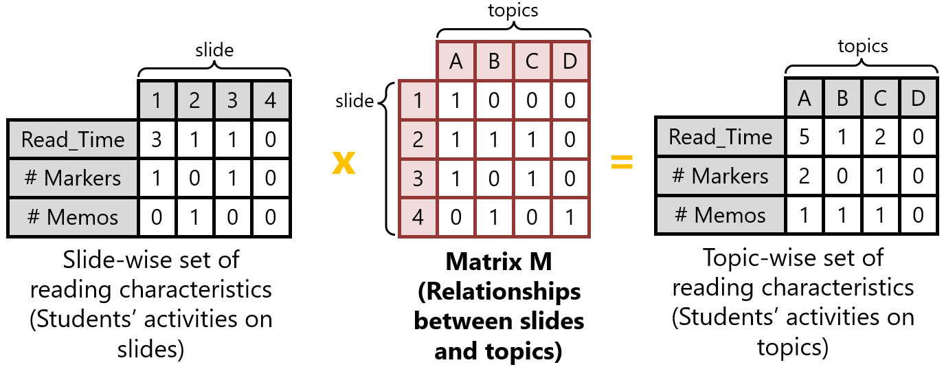
In this context, the present work takes the first step by focusing on the text-processing task. We propose the model LECTOR, which uses Natural Language Processing (NLP) techniques to estimate a quantitative relationship between a lecture slide and a topic. By performing this estimation, we can convert a slide-wise set of reading characteristics into a topic-wise set of reading characteristics (Figure 1). Accordingly, we validate LECTOR’s performance on this task against previous models.
2. RELATED WORK
2.1 Text processing in e-book lecture slides
Previous studies describe the use of e-book lecture slide text to address various problems, such as slide summarization [28], personalized recommendation [21, 23], and learning footprint transfer [33]. Almost all of these works used the TF-IDF method [26] to process their slides [28, 33, 21]. Other works use hierarchical models to perform this process [32, 5], but they require human labeling of all the text in the slides [3], a task that can be burdensome for teachers.
In addition, a previous study estimated topic reading time from e-book user data by considering only the slides where the topic was written [31]. We can reformulate this method as a matrix product (Figure 1), where they assigned a relationship of 1 when the topic appears in a given slide, and 0 in other cases (referred to as “Binary score” in this paper).
2.2 Keyphrase extraction from documents
Our problem is reduced to an unsupervised keyphrase extraction task if we consider lecture slides as documents and topics as key phrases. The state-of-the-art studies on this task use pre-trained models (e.g., Doc2Vec [18], ELMo [25], BERT [12]) to represent words as embedding vectors [6, 29, 13]. Then, their methods estimate the similarity between key phrases and documents from the cosine similarity of their corresponding embedding representations [6, 29, 13].
3. PROPOSED MODEL
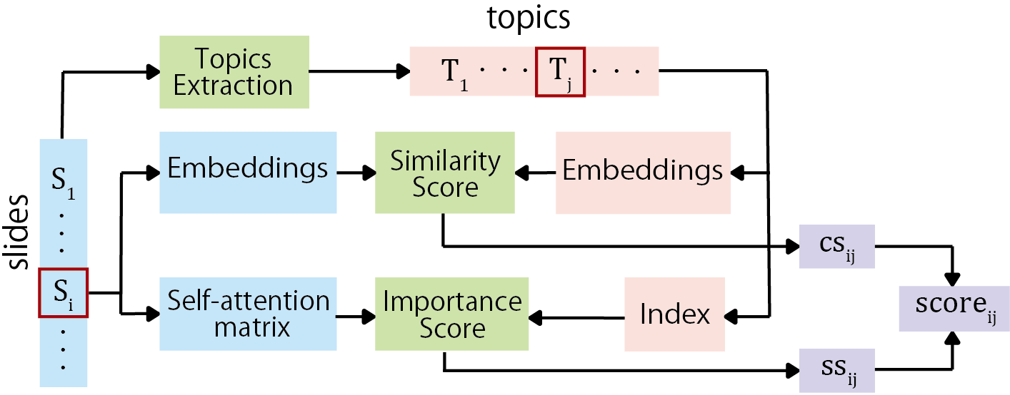
LECTOR extracts a set of topic candidates from all the slides of a given course and assigns a single score to each slide-topic pair (Figure 2). This score is defined as a linear combination of two different scores, one based on the words’ importance and the other on the similarity between the topic and the slide embeddings.
3.1 Topics extraction
We consider a topic to be an observable entity (keyphrase). Models such as EmbedRank [6] and AttentionRank [13] use the Part-Of-Speech to generate noun phrases that become their possible key phrases. In our case, we work with slides written in Japanese and use the Bi-LSTM-based NLP library Nagisa to identify the nouns. Then, we define single nouns and n-gram sequences (n=2) of nouns as our topics.
3.2 Word embeddings and attention matrix
We use a BERT model (fine-tuned on all the course slides’ text in the MLM task [12]) to estimate a self-attention matrix \(A^{i}\) and a set of word embeddings \(E^{i}\) for each slide. We then correct these token-wise values to word-wise values [10].
3.3 LECTOR’s importance score
For a given slide \(s_{i}\), we quantify the attention \(a_{ij}\) that words \(w\) belonging to a given topic \(t_{j}\) receive from all the other words w within the slide \(s_{i}\) by summing the different weights of the matrix \(A^{i}\) as shown in Equation 1. \begin {equation} \label {eq:self-attention summation} a_{ij}=\sum _{w\in t_{j}}\sum _{w'\in s_{i}\setminus \left \{ w \right \}}A_{w'w}^{i} \end {equation} Since this score is strongly influenced by the frequency of the topic’s words \(f_{j}\), the importance score (\(ss_{ij}\)) is calculated by considering the Smooth Inverse Frequency [4] (Equation 2). \begin {equation} \label {eq:sif_weights} ss_{ij}=a_{ij}\left ( \frac {k}{k+f_{j}} \right ) \end {equation}
3.4 LECTOR’s similarity score
For a given slide \(s_{i}\), we estimate its embedding representation \(P_{s}^{i}\) as a weighted average of its corresponding word embeddings \(E^{i}\) (Equation 3). \begin {equation} \label {eq:sentence_embedding} P_{s}^{i}=\sum _{w\in s_{i}}Weight\left ( w \right )E_{w}^{i} \end {equation} We define the word weight as the probability of belonging to the discourse of the given slide. We consider that this discourse is given by a general discourse introduced in the first slide of the lecture material and a specific discourse introduced by the title of the respective slide (Figure 3).
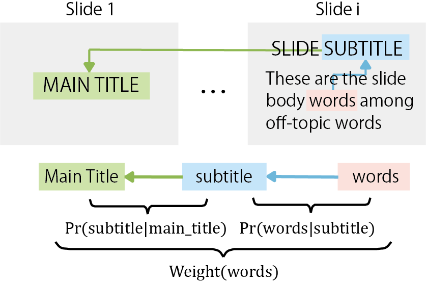
Accordingly, given the set of title and body embeddings \(E_{st}^{i}\) and \(E_{sb}^{i}\), the Weights are calculated as shown in Equation 4. In Appendix A, we detail the formulation and estimation of these Weights from the set of word embeddings. \begin {equation} \label {eq:weight_definition} Weight=Pr\left ( w_{t}\in st_{i}|st_{1} \right )Pr\left ( w_{t}\in sb_{i}|st_{i} \right ) \end {equation} Finally, the similarity score is given by the cosine similarity between the topic \(t_{j}\) and slide \(s_{i}\) embeddings [6, 29, 13]. \begin {equation} \label {eq:cosine_similarity} b_{ij}=\frac {P_{s}^{i} \cdot E_{t}^{j}}{||P_{s}^{i}||\: ||E_{t}^{j}||} \end {equation}
3.5 LECTOR’s final score
The final score for a given topic \(t_{j}\) and slide \(s_{i}\) is a linear combination of the previously normalized importance and similarity scores (Equation 6). The parameter \(d\) defines the importance of each score value. \begin {equation} \label {eq:final_score} score_{ij}=d*ss_{ij}+\left ( 1-d \right )*cs_{ij} \end {equation} LECTOR’s final output is the matrix M, whose elements \(M_{ij}\) are the final scores between slides \(s_{i}\) and topics \(t_{j}\).
4. RESULTS AND DISCUSSION
4.1 Dataset
Our dataset consists of the textual content of 620 slides from 22 e-book materials delivered in the course “Programming Theory” in the year 2019 (before the pandemic restrictions). This course was offered by the School of Engineering at Kyushu University for 7 weeks.
4.2 First Experiment formulation
The ground-truth values to evaluate LECTOR’s estimates are given by the relationships between different topics and slides. However, to find them empirically, we would need a large number of samples because these relationships are perceived differently by different people. Furthermore, given the large number of topics and slides in a course, we would need millions of ground truth labels for each sample.
For this reason, our experiment is designed to indirectly evaluate the estimates of the models. Similar to works on keyphrase extraction, we assume that the most important topics should have the highest relationships with the course content (the different slides). For a given topic \(t_{j}\), we define its keyphrase candidate score \(mt_{j}\) as the sum of the scores obtained across all slides (Equation 7). \begin {equation} \label {eq:exp1_score} mt_{j}=\sum _{i=1}^{\#slides}M_{ij} \end {equation} We use the \(mt_{j}\) values to extract the most important topics of the course. Our ground-truth labels are given by the course keywords extracted from the course syllabus (“Scheme”, “Data Structure”, “List Processing”, “Recursion”, “Expression”, “Condition”, “Design Recipe”, “Function”, “High-level function”). We define @n as the set that contains the top n topics according to the scores \(mt_{j}\). By comparing this set to the ground truth, we can measure the model performance.
We considered three baselines. The first is given by the TF-IDF model [26], which is predominant in the slide text processing literature. The second is given by the AttentionRank model [13], which represents the state-of-the-art in unsupervised keyphrase extraction. The third model is given by the previously described Binary score model proposed by [31].
4.3 First Experiment results
Our results are summarized in Table 1. We can see that AttentionRank outperforms all the other models with an F-score of 28.68% when considering the 5 most important topics. This result shows the high performance of this state-of-the-art model even in a different domain (slides unstructured text). This F-score was achieved by identifying 2 keyphrases in its five most important topics. As we can see in Table 2, while all the models identified the keyphrase “Function” as the most important topic, AttentionRank also identified the keyword “Recursion” as its fourth most important topic. From Table 2, we can also note that despite all the other models achieving the same F-score, the TF-IDF and Binary models are more influenced by the frequency of the topics, estimating topics such as “i" and “define” as one of their most important ones.
| n | Model | P | R | F1 |
|---|---|---|---|---|
|
5 | Baseline (TF-IDF) | 20.00 | 11.11 | 14.39 |
| Baseline (AttentionRank) | 40.00 | 22.22 | 28.68 | |
| Baseline (Binary score) | 20.00 | 11.11 | 14.39 | |
| LECTOR Importance Score | 20.00 | 11.11 | 14.39 | |
| LECTOR Similarity Score | 20.00 | 11.11 | 14.39 | |
| LECTOR | 20.00 | 11.11 | 14.39 | |
|
10 | Baseline (TF-IDF) | 10.00 | 11.11 | 10.63 |
| Baseline (AttentionRank) | 30.00 | 33.33 | 31.68 | |
| Baseline (Binary score) | 10.00 | 11.11 | 10.63 | |
| LECTOR Importance Score | 20.00 | 22.22 | 21.15 | |
| LECTOR Similarity Score | 30.00 | 33.33 | 31.68 | |
| LECTOR | 30.00 | 33.33 | 31.68 | |
|
15 | Baseline (TF-IDF) | 20.00 | 33.33 | 25.11 |
| Baseline (AttentionRank) | 20.00 | 33.33 | 25.11 | |
| Baseline (Binary score) | 20.00 | 33.33 | 25.11 | |
| LECTOR Importance Score | 20.00 | 33.33 | 25.11 | |
| LECTOR Similarity Score | 20.00 | 33.33 | 25.11 | |
| LECTOR | 26.67 | 44.44 | 33.44 | |
Best | Baseline (TF-IDF) | 20.00 | 33.33 | 25.11 |
| Baseline (AttentionRank) | 37.50 | 33.33 | 35.39 | |
| Baseline (Binary score) | 23.08 | 33.33 | 27.38 | |
| LECTOR Importance Score | 20.00 | 33.33 | 25.11 | |
| LECTOR Similarity Score | 25.00 | 44.44 | 32.11 | |
| LECTOR | 33.00 | 44.44 | 38.20 | |
Mean | Baseline (TF-IDF) | 11.68 | 46.00 | 15.53 |
| Baseline (AttentionRank) | 12.63 | 40.89 | 15.65 | |
| Baseline (Binary score) | 11.26 | 43.33 | 14.77 | |
| LECTOR Importance Score | 12.68 | 50.22 | 16.85 | |
| LECTOR Similarity Score | 14.48 | 59.67 | 19.69 | |
| LECTOR | 15.19 | 61.56 | 20.70 |
At \(n=10\), we can see that the attention-based models outperform the TF-IDF and Binary models. Specifically, AttentionRank, LECTOR Similarity score, and LECTOR achieve an F-score of 31.68%. At \(n=15\), LECTOR outperforms all the other models with an F-score of 33.44%. We can see the same result when comparing the best F-score obtained by each model and the mean of the results obtained in the first \(n@100\) sets. These results show that AttentionRank has difficulty finding new keyphrases, whereas LECTOR does not. In Table 2, we can see that AttentionRank tends to give high scores also to minor topics such as “define”, “else”, or “empty” which may explain its lower performance.
| n | TF-IDF | AttentionRank | Binary score | LECTOR
|
|---|---|---|---|---|
| 1 | function | function | function | function |
| 2 | list | example problem | list | data |
| 3 | list (ENG) | definition | define (ENG) | list |
| 4 | i (ENG) | recursion | definition | definition |
| 5 | define (ENG) | example | cond (ENG) | program |
| 6 | definition | value | data | computation |
| 7 | page | define (ENG) | list (ENG) | function definition |
| 8 | data | expression | empty | expression |
| 9 | count | argument | count | example problem |
| 10 | program | computation | i (ENG) | recursion |
| 11 | value | list | value | data definition |
| 12 | expression | else (ENG) | expression | list processing |
| 13 | cond (ENG) | empty (ENG) | recursion | program design |
| 14 | example | element | else (ENG) | recursion function |
| 15 | recursion | count | element | exercises |
The mentioned problem of AttentionRank has two reasons. The first is that its “Accumulated Self-Attention” is influenced by the word frequencies. In their paper, the authors pointed out that this characteristic can be beneficial in large documents. However, in the context of lecture slides, several words from the domain knowledge of the course can appear repeatedly. For example, the mentioned “define” and “else” are well used in the program examples of the course “Programming Theory”. On the other hand, the design we considered in the LECTOR’s importance score limits the influence of the frequency of the words.
However, in the AttentionRank model, topics must also achieve a high "Cross-Attention" value in order to get a high final score. The reason that words like "define" and "else" are important topics of the model is due to the two discourse hypotheses of AttentionRank. For a given slide, the first assumes that the topic candidate defines the slide discourse, and the second assumes that the slide defines the topic discourse. In the context of noisy and unstructured slide text, this consideration can lead to some problems.
For example, given the topic “define” and a slide that contains a programming code example about list processing, the mentioned model will focus on the context words of “define” in the code (including the “define” itself) resulting in a high Cross-attention score in this case. Then, when we consider the topics “list processing” or “example code”, even if the model manages to estimate high scores for these topics, they will be relatively as important as “define”.
Similarly, the presence of noise in the slides can highly influence the relative scores, sometimes estimating low scores for a closely related topic and slide pair. In contrast, LECTOR’s similarity score considers a singular discourse defined by the main title and slide title that give relatively high scores to topics highly related to this discourse. In the previous example, LECTOR would give higher scores to “list processing” and “example code” rather than “define”, and also would give a higher score to “define” rather than a random noise word.
4.4 Second Experiment formulation
Previous studies of students’ eye-tracking data have concluded that each student has a different preference for learning content [20]. Accordingly, this experiment aims to compare the topic preferences of students with different grades.
We extract their reading time on the different slides (inside and outside of class) and obtain their slide preferences by normalizing the reading time values across the week. Then, we use LECTOR to quantify their Relative Reading Times for the different topics (Topic RRT), as shown in Figure 1. Finally, we group the students according to their grades (A=24, B=6, C=4, D=6, F=10) and compare both their reading time and RRT distributions. We measure the separability of the distributions by using the Fisher Discriminant Ratio (FDR) and statistically validated them with a T-test.
| A-B | B-C | C-D | D-F | At-risk | ||
|---|---|---|---|---|---|---|
WEEK 1 (IN-CLASS) | Reading Time | 0.0342 | 0.2615 | 2.782 | 0.0229 | 1.111* |
| Topic RRT | 1.4517 | 612.44* | 46.861 | 3.233* | 4.3245 | |
| (Topic) | (expressions) | (data) | (exercises) | (design | (execution) | |
| method) | ||||||
WEEK 1 (OUT-CLASS) | Reading Time | 0.0409 | 0.0023 | 0.0436 | 0.0085 | 0.000 |
| Topic RRT | 3.0031 | 29.3069 | 653.11** | 72.649 | 1.4049 | |
| (Topic) | (auxiliary | (problems) | (program | (problems) | (auxiliary | |
| functions) | design) | functions) | ||||
WEEK 2 (IN-CLASS) | Reading Time | 1.0128 | 0.6902 | 0.1735 | 0.0021 | 0.0192 |
| Topic RRT | 6.3908 | 8.4876 | 568.83* | 1.7794 | 1.5921 | |
| (Topic) | (problems) | (boolean | (problems) | (program) | (program) | |
| value) | ||||||
WEEK 2 (OUT-CLASS) | Reading Time | 0.0502 | 0.0855 | 0.2629 | 0.0913 | 0.325* |
| Topic RRT | 5.5802* | 29.9718 | 241.1* | 2.8445 | 17.92* | |
| (Topic) | (design | (cond | (data | (body | (exercise | |
| method) | expression) | analysis) | expression) | problems) | ||
WEEK 3 (IN-CLASS) | Reading Time | 0.0503 | 0.4597 | 0.1141 | 0.0142 | 0.3367 |
| Topic RRT | 11.8214 | 8.263 | 7.998 | 15.061 | 5.031 | |
| (Topic) | (exercise | (synthetic | (synthetic | (sorting) | (examples) | |
| problems) | data) | data) | ||||
WEEK 3 (OUT-CLASS) | Reading Time | 0.0234 | 0.0008 | 0.2131 | 1.4279 | 0.1951 |
| Topic RRT | 15.166* | 168.33* | 286.84** | 42.266 | 43.126* | |
| (Topic) | (templates) | (element | (structure | (exercice | (exercice | |
| count) | element) | problems) | problems) | |||
*p<0.05 **p<0.01 |
4.5 Second Experiment results
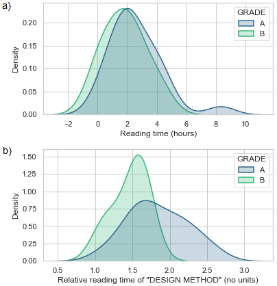
We can see an example of our results in Figure 4. Figure 4a shows the distribution of the reading time of the students with final grades A and B in the second week after the lecture (out-class). Both distributions overlap, so the FDR is 0.0502 and the significance level (p) of the T-test is 0.3302. In Figure 4b we see the same distributions when we consider the relative time spent reading about “Design method”. Here, students with a final grade of A tend to read more on this topic, resulting in a higher FDR of 5.5802 and a lower p of 0.037 in the T-test.
Our different results are summarized in Table 3. We considered the first 3 weeks of the course because of insufficient data in later weeks due to dropouts. As shown in this table, we have included 5 cases, comparing students with consecutive grades (A-B, B-C, C-D, D-F) and at-risk students (students who failed the course) with non-risk students. The result shown in Figure 4 can be found in the first column and fourth row of the table.
In the results of Reading Time, we can see that students from different groups tend to read the same amount of time. In the case of at-risk and non-risk student groups, we find statistically significant differences in out-of-class engagement in the second and third weeks. On the other hand, we find statistically significant differences between different groups almost 40% of the time when we consider the Topic RRT, which means that these preferences are good variables to understand the differences between students with different grades. This suggests that works that attempt to predict at-risk students such as [24, 8] may benefit from the integration of models such as LECTOR to obtain more differentiated features.
We can consider student’s reading preferences for further analysis. For example, as mentioned earlier, at-risk students engage less outside of class in the second and third weeks. In Table 3, we also see that they tend to focus more on exercise problems. This is a signal that at-risk students adopt a surface learning approach [17], focusing on the content directly related to the assessments. Thus, previous works [1, 34] that have analyzed the students’ reading behavior can use the topic preferences to make better reports.
5. LIMITATIONS
The first limitation is the indirect evaluation of the models’ estimates. As previously discussed, collecting labels for a direct evaluation is impractical, but if we limit the number of topics to the most important ones we can collect a limited set of labels to conduct a more direct evaluation.
The second limitation is the size of our dataset. To evaluate the generalizability of our model, we need to consider slides from different courses. In a science course, the slides are less structured and include equations or code. In this case, the robustness of LECTOR plays an important role. In addition, our slides are in Japanese and the generality of our results may be affected by the use of other methods for topic extraction in different languages.
6. CONCLUSIONS
We proposed LECTOR, a new model that adapts state-of-the-art keyphrase extraction models to the domain of lecture slides. From our results, we conclude that LECTOR can quantitatively extract the relationships between topics and e-book lecture slides better than previous models when considering noisy text from scientific lecture slides. LECTOR was able to extract important topics (higher F-score) while avoiding frequent out-of-context topics.
LECTOR’s topic-wise representation of e-book reading characteristics provides new insights into the students reading behavior. Specifically, it allows to access the students’ preferences for some topics and use them to model more detailed behaviors. Our results show that this new model preserves the differences related to reading preferences that exist between students with different final grades.
These responses validate the benefits of integrating attention-based models like LECTOR into reading behavior models. Accordingly, it allows future works to consider students reading preferences in their models. Also, our model can be used for other text processing tasks, such as slide summarization, content recommendation, etc.
7. ACKNOWLEDGMENTS
This work was supported by JST CREST Grant Number JPMJCR22D1 and JSPS KAKENHI Grant Number JP22H00551, Japan.
8. REFERENCES
- G. Akçapinar, M.-R. A. Chen, R. Majumdar, B. Flanagan, and H. Ogata. Exploring Student Approaches to Learning through Sequence Analysis of Reading Logs, page 106–111. Association for Computing Machinery, New York, NY, USA, 2020.
- G. Akçapinar, M. N. Hasnine, R. Majumdar, B. Flanagan, and H. Ogata. Developing an early-warning system for spotting at-risk students by using ebook interaction logs. Smart Learning Environments, 6(1):4, May 2019.
- F. N. Al-Aswadi, H. Y. Chan, and K. H. Gan. Automatic ontology construction from text: a review from shallow to deep learning trend. Artificial Intelligence Review, 53(6):3901–3928, Aug 2020.
- S. Arora, Y. Liang, and T. Ma. A simple but tough-to-beat baseline for sentence embeddings. In International Conference on Learning Representations, 2017.
- T. Atapattu, K. Falkner, and N. Falkner. A comprehensive text analysis of lecture slides to generate concept maps. Computers & Education, 115:96–113, 2017.
- K. Bennani-Smires, C. Musat, A. Hossmann, M. Baeriswyl, and M. Jaggi. Simple unsupervised keyphrase extraction using sentence embeddings. In Proceedings of the 22nd Conference on Computational Natural Language Learning, pages 221–229, Brussels, Belgium, Oct. 2018. Association for Computational Linguistics.
- P. Blikstein and M. Worsley. Multimodal learning analytics and education data mining: using computational technologies to measure complex learning tasks. Journal of Learning Analytics, 3(2):220–238, Sep. 2016.
- C.-H. Chen, S. J. H. Yang, J.-X. Weng, H. Ogata, and C.-Y. Su. Predicting at-risk university students based on their e-book reading behaviours by using machine learning classifiers. Australasian Journal of Educational Technology, 37(4):130–144, Jun. 2021.
- S. K. Cheung, J. Lam, N.Lau, and C.Shim. Instructional design practices for blended learning. In 2010 International Conference on Computational Intelligence and Software Engineering, pages 1–4, 2010.
- K. Clark, U. Khandelwal, O. Levy, and C. D. Manning. What does BERT look at? an analysis of BERT’s attention. In Proceedings of the 2019 ACL Workshop BlackboxNLP: Analyzing and Interpreting Neural Networks for NLP, pages 276–286, Florence, Italy, Aug. 2019. Association for Computational Linguistics.
- Y. Cui, Z. Chen, S. Wei, S. Wang, T. Liu, and G. Hu. Attention-over-attention neural networks for reading comprehension. In Proceedings of the 55th Annual Meeting of the Association for Computational Linguistics (Volume 1: Long Papers), pages 593–602, Vancouver, Canada, July 2017. Association for Computational Linguistics.
- J. Devlin, M.-W. Chang, K. Lee, and K. Toutanova. BERT: Pre-training of deep bidirectional transformers for language understanding. In Proceedings of the 2019 Conference of the North American Chapter of the Association for Computational Linguistics: Human Language Technologies, Volume 1 (Long and Short Papers), pages 4171–4186, Minneapolis, Minnesota, June 2019. Association for Computational Linguistics.
- H. Ding and X. Luo. AttentionRank: Unsupervised keyphrase extraction using self and cross attentions. In Proceedings of the 2021 Conference on Empirical Methods in Natural Language Processing, pages 1919–1928, Online and Punta Cana, Dominican Republic, Nov. 2021. Association for Computational Linguistics.
- B. Flanagan and H. Ogata. Integration of learning analytics research and production systems while protecting privacy. In Workshop Proceedings of the 25th International Conference on Computers in Education, pages 355–360, 12 2017.
- B. Flanagan and H. Ogata. Learning analytics platform in higher education in japan. Knowledge Management and E-Learning, 10:469–484, 11 2018.
- F. Martin, A. Ritzhaupt, S. Kumar, and K. Budhrani. Award-winning faculty online teaching practices: Course design, assessment and evaluation, and facilitation. The Internet and Higher Education, 42:34–43, 2019.
- F. Marton and R. Säaljö. On qualitative differences in learning—ii outcome as a function of the learner’s conception of the task. British Journal of Educational Psychology, 46(2):115–127, 1976.
- T. Mikolov, I. Sutskever, K. Chen, G. S. Corrado, and J. Dean. Distributed representations of words and phrases and their compositionality. In C. Burges, L. Bottou, M. Welling, Z. Ghahramani, and K. Weinberger, editors, Advances in Neural Information Processing Systems, volume 26, pages 3111–3119. Curran Associates, Inc., 2013.
- A. Mnih and G. Hinton. Three new graphical models for statistical language modelling. In Proceedings of the 24th International Conference on Machine Learning, ICML ’07, page 641–648, New York, NY, USA, 2007. Association for Computing Machinery.
- S. Mu, M. Cui, X. J. Wang, J. X. Qiao, and D. M. Tang. Learners’ attention preferences of information in online learning. Interactive Technology and Smart Education, 16(3):186–203, Jan 2019.
- K. Nakayama, M. Yamada, A. Shimada, T. Minematsu, and R. ichiro Taniguchi. Learning support system for providing page-wise recommendation in e-textbooks. In K. Graziano, editor, Proceedings of Society for Information Technology & Teacher Education International Conference 2019, pages 1078–1085, Las Vegas, NV, United States, March 2019. Association for the Advancement of Computing in Education (AACE).
- H. Ogata, M. Oi, K. Mohri, F. Okubo, A. Shimada, M. Yamada, J. Wang, and S. Hirokawa. Learning analytics for E-book-based educational big data in higher education, pages 327–350. Springer International Publishing, May 2017.
- F. Okubo, T. Shiino, T. Minematsu, Y. Taniguchi, and A. Shimada. Adaptive learning support system based on automatic recommendation of personalized review materials. IEEE Transactions on Learning Technologies, 16(1):92–105, 2023.
- F. Okubo, T. Yamashita, A. Shimada, Y. Taniguchi, and K. Shin’ichi. On the prediction of students’ quiz score by recurrent neural network. CEUR Workshop Proceedings, 2163, 2018.
- M. E. Peters, M. Neumann, M. Iyyer, M. Gardner, C. Clark, K. Lee, and L. Zettlemoyer. Deep contextualized word representations. In Proceedings of the 2018 Conference of the North American Chapter of the Association for Computational Linguistics: Human Language Technologies, Volume 1 (Long Papers), pages 2227–2237, New Orleans, Louisiana, June 2018. Association for Computational Linguistics.
- G. Salton and C. Buckley. Term-weighting approaches in automatic text retrieval. Information Processing & Management, 24(5):513–523, 1988.
- G. Sedrakyan, J. Malmberg, K. Verbert, S. Järvelä, and P. A. Kirschner. Linking learning behavior analytics and learning science concepts: Designing a learning analytics dashboard for feedback to support learning regulation. Computers in Human Behavior, 107:105512, 2020.
- A. Shimada, F. Okubo, C. Yin, and H. Ogata. Automatic summarization of lecture slides for enhanced student previewtechnical report and user study. IEEE Transactions on Learning Technologies, 11(2):165–178, 2018.
- Y. Sun, H. Qiu, Y. Zheng, Z. Wang, and C. Zhang. Sifrank: A new baseline for unsupervised keyphrase extraction based on pre-trained language model. IEEE Access, 8:10896–10906, 2020.
- A. Vaswani, N. Shazeer, N. Parmar, J. Uszkoreit, L. Jones, A. N. Gomez, L. ukasz Kaiser, and I. Polosukhin. Attention is all you need. In I. Guyon, U. V. Luxburg, S. Bengio, H. Wallach, R. Fergus, S. Vishwanathan, and R. Garnett, editors, Advances in Neural Information Processing Systems, volume 30, pages 5998–6008. Curran Associates, Inc., 2017.
- J. Wang, T. Minematsu, Y. Taniguchi, F. Okubo, and A. Shimada. Topic-based representation of learning activities for new learning pattern analytics. In Proceedings of the 30th International Conference on Computers in Education, pages 268–378, 12 2022.
- Y. Wang and K. Sumiya. Semantic ranking of lecture slides based on conceptual relationship and presentational structure. Procedia Computer Science, 1(2):2801–2810, 2010. Proceedings of the 1st Workshop on Recommender Systems for Technology Enhanced Learning (RecSysTEL 2010).
- C. Yang, B. Flanagan, G. Akcapinar, and H. Ogata. Maintaining reading experience continuity across e-book revisions. Research and Practice in Technology Enhanced Learning, 13(1):24, Dec 2018.
- C. Yin, M. Yamada, M. Oi, A. Shimada, F. Okubo, K. Kojima, and H. Ogata. Exploring the relationships between reading behavior patterns and learning outcomes based on log data from e-books: A human factor approach. International Journal of Human–Computer Interaction, 35(4-5):313–322, 2019.
APPENDIX
A. WORDS’ WEIGHTS ESTIMATION
A.1 Preliminary definition
Given a set of words \(A=\{w_{a}^{1},w_{a}^{2},..\}\) and \(B=\{w_{b}^{1},w_{b}^{2},..\}\), we will estimate \(Pr\left ( w_{a}\in A|B \right )\): The probability of each word in A being generated under the discourse (context) of the set of words B.
First, the probability that a given word \(w_{a}\) is generated under a given context word \(w_{b}\) is proportional to the inner product of their word embeddings (Equation 8) [4, 19]. \begin {equation} \label {eq:prob_dot_product} Pr\left ( w_{a} | w_{b} \right )\propto exp\left ( e_{a} \cdot e_{b}^{T} \right ) \end {equation} With this equation, we can estimate the probability of each word \(w_{a}\) in the set \(A\) to be generated under the single context word \(w_{b}\), as shown in Equation 9. \begin {equation} \label {eq:prob_dot_product_gen} Pr\left ( w_{a} \in A| w_{b} \right )= [ k_{1}exp{\left ( e_{a} \cdot e_{b}^{T} \right )}, k_{2}exp\left ( e_{a} \cdot e_{b}^{T} \right ),..] \end {equation} We assume a common proportional constant (\(k_{1}=k_{2}=...\)). Then, we can represent Equation 9 as the softmax of the matrix product between the set of embeddings \(E_a = [e_{a}^{1},e_{a}^{2},..]\) and the context embedding \(e_b\), as shown in Equation 10 (the parameter \(\varphi \) preserves the influence of the proportional constant). This equation can also be interpreted as the cross-attention between the Query \(e_{b}\) and the Key \(E_{a}\) [30]. \begin {equation} \label {eq:probability_given_context} Pr\left ( w_{a}\in A|w_{b} \right )=Softmax\left ( \frac {e_{b}\cdot {E_{a}}^{T}}{\varphi } \right ) \end {equation} Finally, we can generalize this equation to the context \(B = \{w_{b}^{1},w_{b}^{2},...\}\) by using the approach “Attention over attention” proposed in the study [11]. \begin {equation} \label {eq:s_matrix_definition} S=\frac {E_{b}\cdot {E_{a}}^{T}}{\varphi } \end {equation} \begin {equation} \label {eq:generalized_probability} Pr\left ( w_{a}\in A|B \right )={AV_{row}}\left ( SF_{col}\left ( S \right ) \right )SF_{row}\left ( S \right ) \end {equation} where \(AV_{row}\) means average along the row axis, \(SF_{col}\) means softmax along the column axis, and \(SF_{row}\) means softmax along the row axis.
A.2 Formulation
Given the set of words embeddings \(E_{i}\) for each slide, we split it into the set of title and body embeddings \(E_{st}^{i}\) and \(E_{sb}^{i}\). Then, the words’ Weights are estimated using Equations 10 and 12 as follows: \begin {equation} \label {eq:s_matrix_weight} S=\frac {E_{st}^{1}\cdot {E_{st}^{i}}^{T}}{\varphi } \end {equation} \begin {equation} \label {eq:generalized_weight} Pr\left ( w_{t}\in st_{i}|st_{1} \right )={AV_{row}}\left ( SF_{col}\left ( S \right ) \right )SF_{row}\left ( S \right ) \end {equation} \begin {equation} \label {eq:prev_weight} Pr\left ( w_{t}\in sb_{i}|st_{i} \right )=Softmax\left ( \frac {E_{st}^{i}\cdot {E_{sb}^{i}}^{T}}{\varphi } \right ) \end {equation} \begin {equation} \label {eq:weight_definition_one_more} Weight=Pr\left ( w_{t}\in st_{i}|st_{1} \right )Pr\left ( w_{t}\in sb_{i}|st_{i} \right ) \end {equation}
© 2023 Copyright is held by the author(s). This work is distributed under the Creative Commons Attribution-NonCommercial-NoDerivatives 4.0 International (CC BY-NC-ND 4.0) license.