ABSTRACT
Problem decomposition into sub-problems or subgoals and recomposition of the solutions to the subgoals into one complete solution is a common strategy to reduce difficulties in structured problem solving. In this study, we use a data-driven graph-mining-based method to decompose historical student solutions of logic-proof problems into Chunks. We design a new problem type where we present these chunks in a Parsons Problem fashion and asked students to reconstruct the complete solution from the chunks. We incorporated these problems within an intelligent logic tutor and called them Chunky Parsons Problems (CPP). These problems demonstrate the process of problem decomposition to students and require them to pay attention to the decomposed solution while they reconstruct the complete solution. The aim of introducing CPP was to improve students’ problem-solving skills and performance by improving their decomposition-recomposition skills without significantly increasing training difficulty. Our analysis showed that CPPs could be as easy as Worked Examples (WE). And, students who received CPP with simple explanations attached to the chunks had marginally higher scores than those who received CPPs without explanation or did not receive them. Also, the normalized learning gain of these students shifted more towards the positive side than other students. Finally, as we looked into their proof-construction traces in posttest problems, we observed them to form identifiable chunks aligned with those found in historical solutions with higher efficiency.
Keywords
1. INTRODUCTION
Computational thinking, a set of skills and practices for
complex problem solving, provides a foundation for learning
21st-century skills, particularly computer science (CS).
Educational researchers and teaching professionals acknowledge
problem decomposition-recomposition skill as a key component
of computational thinking and complex problem solving
[11, 23, 13, 22]. Efficient problem solving using the problem
decomposition skill or strategy involves several steps: 1)
identifying sub-problems (i.e. subgoals) to reduce the difficulty
associated with the problem, 2) constructing a solution for each
of those sub-problems, and 3) recomposing the sub-problem
solutions to form the larger solution [5]. Research showed that
experts carry out problem decomposition and recomposition
(PDR) steps more than novices [41]. However, several
studies also showed that novices often attempt to decompose
problems [26, 40]. But while they may demonstrate correct
decomposition in easier problems, novices fail to decompose
sophisticated problems [26].
Despite problem decomposition-recomposition (PDR) being
vital to complex problem-solving, it is rarely mentioned
explicitly in instructional materials for computer science (a discipline focused on complex problem solving using computers)
[30]. Also, existing research lacks guidance on how to
motivate students to adopt this PDR process or how to
improve their skills associated with PDR. A few studies
analyzed the differences between experts and novices in
adopting this PDR process, indicating that experts use
PDR more than novices [27, 20]. And, a few studies aimed
at introducing this PDR skill to students, mostly during
programming problem solving, using varying methods [for
example, using pattern-oriented instruction [32], programming
problem decomposition exercise [42], guided inquiry-based
instruction [36], etc.]. However, PDR remains under-explored in
the instruction of other structured problem-solving domains.
In this study, we design, implement, and evaluate a problem-based
training intervention, named Chunky Parsons Problem
(CPP), that introduces to students the concept of problem
decomposition-recomposition (PDR) while engaging them in
these processes during problem solving within an intelligent
logic tutor, DT (Deep Thought). To generate CPP, we
decomposed students’ historical solutions to each logic-proof
construction problem stored in DT’s problem bank into
sub-proofs (referred to as chunks) using a data-driven method.
These chunks are presented in a Parsons Problem fashion. In a
traditional Parsons Problem, all steps contributing to the
complete solution of a problem are presented in a jumbled
order. On the contrary, within CPP, the solution to a logic-proof
problem is presented as jumbled-up chunks (groups of connected
statements) instead of individual statements. By design, CPP is
a partially worked example where all the required statements
are shown in chunks. However, the missing connections
among the chunks give the students an opportunity to
recompose the solution while having them pay attention to the
decomposition to understand the composition of each chunk,
how each chunk contributes to other chunks, and the overall
solution. Thus, CPPs can be thought of as problems that are
partially worked-examples and partially problem-solving (PS)
problems.
We deployed DT with CPP implemented within its training
session in an undergraduate classroom of CS majors and
conducted a controlled experiment. In the controlled experiment,
we implemented three training conditions: 1) Control(C):
received only worked example (WE) and problem-solving (PS)
logic-proof construction problems, 2) Treatment 1(\(T_1\)): received
CPP (without explicit explanation of the chunks) along with
PS/WE, and 3) group who receive CPP (with explicit
explanation attached to the chunks) along with PS/WE. Since
prior research showed that explicit instruction on what to learn
or take away from an intervention may help to improve
students’ decomposition ability [36], we introduced the last
training condition to identify the more effective representation
(between with/without explanation) of CPP. Finally, we
evaluated the efficacy of CPP by answering the following
research questions:
- RQ1: How do Chunky Parsons Problems impact students’ performance and learning?
- RQ2: What are the difficulties associated with solving a Chunky Parsons Problem?
- RQ3: How do Chunky Parsons Problems impact students’ Chunking (problem decomposition-recomposition) behavior and skills while solving a new problem?
2. BACKGROUND AND MOTIVATION
Existing research has identified problem decomposition-recomposition
(PDR) as difficult for novices as problems get more complex [26].
However, we found only a few studies investigating methods to
improve this skill. For example, Pearce et al. [36] explored
explicit instruction (openly instructing students to learn
problem decomposition and describing how to go about that
learning) to improve students’ problem decomposition
skills and concluded that explicit instruction can lead to
significant gains in mastering this skill. Muller et al. [32]
found that pattern-oriented instruction can have a positive
impact on problem decomposition skills. We found some
studies where researchers in the domain of mathematics and
programming, using problem-based methods, aimed at
improving students’ subgoal learning which is equivalent to the
skill of identifying sub-tasks required to solve a problem (i.e.
problem decomposition). The most common method explored
by researchers in this regard is subgoal-labeled worked
examples or instructional materials [29, 8, 7]. Studies
showed that worked examples with abstract labels that
give away structural information help improve students’
problem-solving skills measured by test scores. However.
these studies do not evaluate or measure students’ problem
decomposition or subgoaling skills after training. Also, we did
not find any established guidance on how problem-based
interventions can be generated automatically and how they
should be designed to be used within tutors to improve
students’ problem decomposition-recomposition (or chunking)
skills.
From our literature review, we concluded that problem-based
interventions specifically designed for tutors to improve
students’ chunking skills are under-explored. Thus, in this
paper, we set our aim to design and implement CPPs to be used
within DT to improve students’ problem-solving and chunking
skills. While extracting chunks to present within CPP and
designing its representation within DT, we considered three
goals: 1) Automating the solution-decomposition process
to extract chunks so that expert effort is not required;
2) Designing the problem to demonstrate chunking and
engaging students in the process to improve their skills, and
3) keeping the difficulty-level low so that students can
persist and learn. To set the difficulty level of our problem,
we explored problem types that are of low difficulty as
established by literature: Worked Examples and Parsons
Problems.
Worked Examples: Worked examples (WE) reduce learners’ intrinsic load (i.e. working memory load which is caused by the
complexity of the problem) and help them to learn better [35].
This improvement in learning due to worked examples is
referred to as the Worked Example Effect [44] in literature.
However, several studies argued the applicability of worked
examples in certain situations. For example, worked examples
may not be useful for students with high prior knowledge [34],
when problems are structured [34], or if the problem is strategic
but involves only a few interactive elements [10]. In such cases,
problem-solving (PS) supports the learning process better [10].
Also, for goal or product-directed problems, a worked example
only shows the construction of the solution and does not help
students to grow an understanding of the rationale behind the
selection of certain steps [49]. In this scenario, students fail to
acquire a schema of the problem-solving approach which leads
to the failure to transfer problem-solving skills. Renkl et
al. [39] suggested that worked examples help students to
learn better only when the examples give away structural
information of the solution and isolate meaningful building
blocks.
Parsons Problems: Parsons problems ask students to construct a
solution from a given set of jumbled solution steps [14]. Poulsen
et al. showed the application of the Parsons problem in a
mathematical proof construction tool, Proof Blocks [38]. They
found that Parsons Problems within Proof Blocks significantly
reduced the difficulty associated with proof construction.
Parsons problem is heavily explored in programming education.
Studies found that Parsons problems can improve students’ code
writing capability [48, 24, 14, 17] or can help in completing
programming tasks efficiently without impacting performance
on subsequent programming tasks [51]. Studies also showed that
attached explanations [18] and subgoal labels [31] can help
students solve Parsons problem and improve the learning
process.
From the overview of the impact of WEs and Parsons Problem,
we designed CPPs as partially WE and partially PS, which
represent meaningful building blocks of a proof (i.e. Chunks) in
a Parsons Problem fashion. Additionally, we explored attaching
explanations to the chunks to further reduce difficulties and
support students’ learning process.
Data-driven Solution Decomposition Techniques: Data-driven
solution decomposition refers to the process of automatically
decomposing a problem or its solution into subgoals or
sub-solutions based on the properties found in historical
solutions. These historical solutions often come from tutors or
learning platforms that collect students’ solution traces and
thus, are often redundant. While performing data-driven
decomposition, researchers mainly focused on identifying
independent or dependent components of a solution. To
do so, they often presented student solutions as graphs
depicting how they moved from state to state to reach the final
solution [37, 50, 45, 33, 4]. Prior research showed the
application of clustering [37] or connected component
detection [50, 45, 16] to extract independent sub-solutions or
chunks in these graphical models. On the other hand, some
researchers [12, 19] proposed constraint-based decomposition
techniques for linear problem solutions such that decomposed
sub-solutions can be replaced with alternate solutions without
causing any problem. To decompose computer programs,
researchers have used methods where they looked at the usage
of different program components (for ex., variables) to identify
independent parts of the program [46, 47]. In this paper,
we demonstrate a solution decomposition method that
extracts chunks by applying rules/constraints on graphical
representations of historical student solutions similar to Eagle et
al.’s work [16].
Evaluation of Students’ Chunking Skills We observed that in
prior research, researchers have only used test scores to evaluate
methods that were set to teach students chunking/PDR. Only a
few recent studies explored methods to measure students’
chunking skills from data. Kwon and Cheon [26] mapped
predefined sub-tasks and program segments in Scratch
programs to observe how students decompose and develop
programs. In a recent study, Charitsis et al. [9] used NLP to
identify key components and students’ approaches to develop
programs and then relate those to performance metrics using
linear regression to quantify their decomposition skills.
Kinnebrew et al. [25] also mined frequent patterns in students’
action sequences and relate that to performance to explain
their learning behavior. Overall, to evaluate decomposition
skills, these studies each sought a baseline to compare
students’ solutions against and explained performance using
solution characteristics. In this paper, to measure students’
chunking/PDR skills after being trained with CPPs, we
analyzed students’ step sequences during proof construction to
identify potential chunking/PDR instances and tried to
explain their performance through the chunking/PDR
characteristics.
3. METHOD
In this study, we explored Chunky Parsons Problems (with or without explicit explanations attached to them) to improve students’ problem-solving skills (with an emphasis on Chunking/PDR skills) and learning gain in the context of logic-proof problems. We derived CPP using a data-driven method and incorporated them into the training session within DT [28], an intelligent logic tutor. In the subsequent sections, we first provide a brief introduction to DT. Then, we discuss how we derived CPP from data, designed explanations explaining the chunks, and presented them within DT. Finally, we present the design of our experimental training conditions and data collection method to facilitate analyses to answer our research questions
3.1 Deep Thought (DT), the Intelligent Logic Tutor
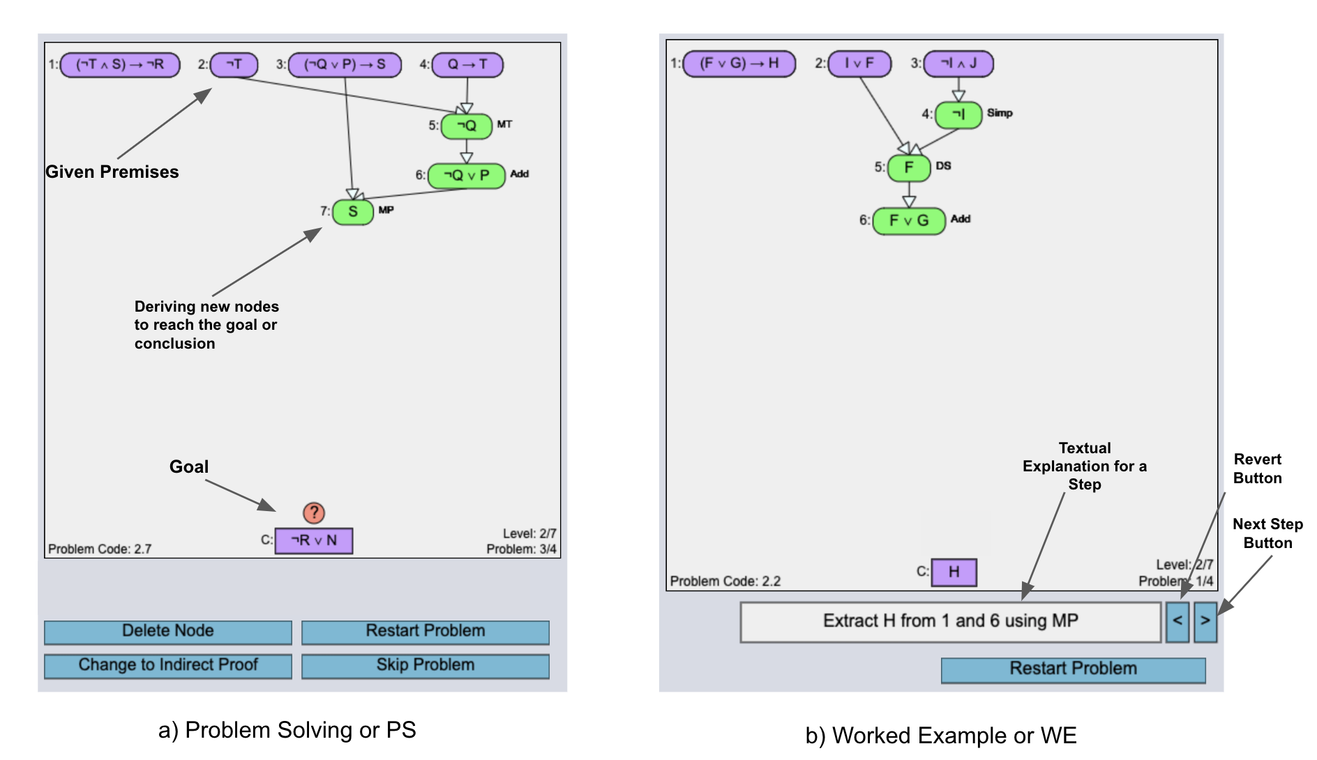
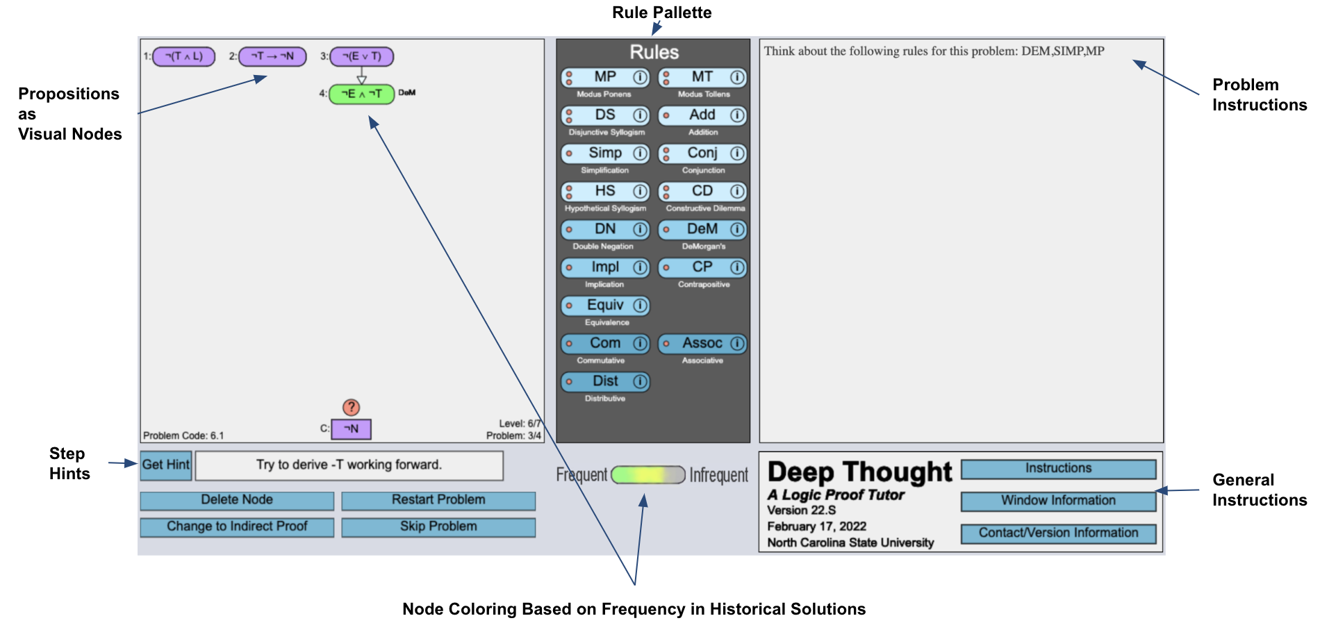
DT is an intelligent logic tutor that teaches students logic-proof
construction. Each logic-proof problem within DT contains a set
of given premises and a conclusion presented as visual nodes
[Figure 1a]. To solve a problem, new propositions (or nodes) are
needed to be derived by applying valid logic rules on the given
premises and subsequently on derived premises to reach the
conclusion. Usually, each problem in DT is either of type
Worked Example (WE) or problem-solving (PS). WEs
are solved by the tutor step-by-step as the students click
on a next step (\(>\)) button [Figure 1b]. On the other hand,
PSs are required to be solved by the students where they have to derive all the steps of a proof [Figure 1a]. Here,
a step refers to the process of deriving a single node or
proposition.
DT is organized into 7 levels. In the first level, the tutor starts
by showing two sample logic-proof problems (one WE and one
PS) to help students understand how to use different features of
the tutor. Then, the students solve two pretest PS problems.
After the pretest level (i.e. level 1), the students go through 5
training levels with 4 problems in each level. Each of the first
three problems in the training levels is either a WE or PS. For
these training-level PS problems, on-demand step-level
hints are available. The last problem in each training level
is always of type PS and is called the training-level test
problem. After the 5 training levels, students enter into
a posttest level containing 6 PS problems. During the
pretest, training-level test, and posttest problems, the tutor
does not offer any hints or help and the students have to
solve them independently. For each of these problems,
students receive a score between 0 and 100 (efficient proof
construction [less time, fewer step counts, and incorrect rule
applications] receives higher scores) [3, 1]. The pretest
scores represent students’ mastery level before training. On
the other hand, the training-level posttest and posttest
scores track how much students learned after each level of
training and after all 5 training levels. More Details on
DT interface and features can be found in Appendix A.
3.2 Deriving Chunky Parsons Problem (CPP)
using a data-driven Graph-Mining
Approach
Data for Deriving CPP: DT has been being deployed in an
undergraduate logic course offered at a public research
university in the Fall and Spring semesters since 2012. To derive
CPP representation for logic proofs, we used the most
recent log data collected by DT in the Fall and Spring
of the years 2018-2021. These log data detail students’
historical step-by-step proof-construction attempts for
each problem they solved within DT. Using these data, we
generated high-level graphical representations (Interaction
Networks [16] and Approach Maps [15]) of students’ solution
approaches for these problems to derive CPP from them. For
each problem, data of approximately 170-200 students
containing altogether 2000-5500 solution steps were used. To
select the students, we performed equal random sampling
from the semesters mentioned before so that the data is
representative of different student groups who took the
course over the years. The reason for not using all data is to
mainly reduce the computational complexity of the adopted
graph mining approach. Also, the data used is assumed
sufficient enough to capture common student approaches to
solve each logic-proof problem in the problem bank of
DT [43].
Interaction Network and Approach Map: For each of the
problems in the DT problem bank, we generated a graphical
representation of how students moved from one state to another
during the construction of a proof for the problem. Here, a
state refers to all nodes (or propositions) a student had
at a particular moment during their proof construction
attempt. Students move from state to state by deriving or
deleting nodes, i.e. via a step. To limit the number of states
in the graph, the propositions at a particular state are
lexicographically ordered, which means that the order of
derivation of the nodes is not considered in the graphical
representation. This graphical representation of students’
proof-construction attempts for a problem is called an
interaction network since it represents the interaction among
the states [16]. Since interaction networks are often very large
and visually uninterpretable, we applied Girvan-Newman
community clustering [21] on the interaction networks to
identify regions or clusters of closely connected states. Each
cluster contains a set of states containing effective propositions
that contributed to the final proof submitted by the students
and also unnecessary propositions (i.e. propositions that did not
contribute to the final proof) that they derived along the way.
We represented each cluster with one single graphical node
containing only the effective propositions. Thus, we obtained a
graph where the start state containing the given premises is
connected to the conclusion through clusters of effective
propositions. Each path from start to conclusion represents one
student approach (or solution) to the logic-proof problem
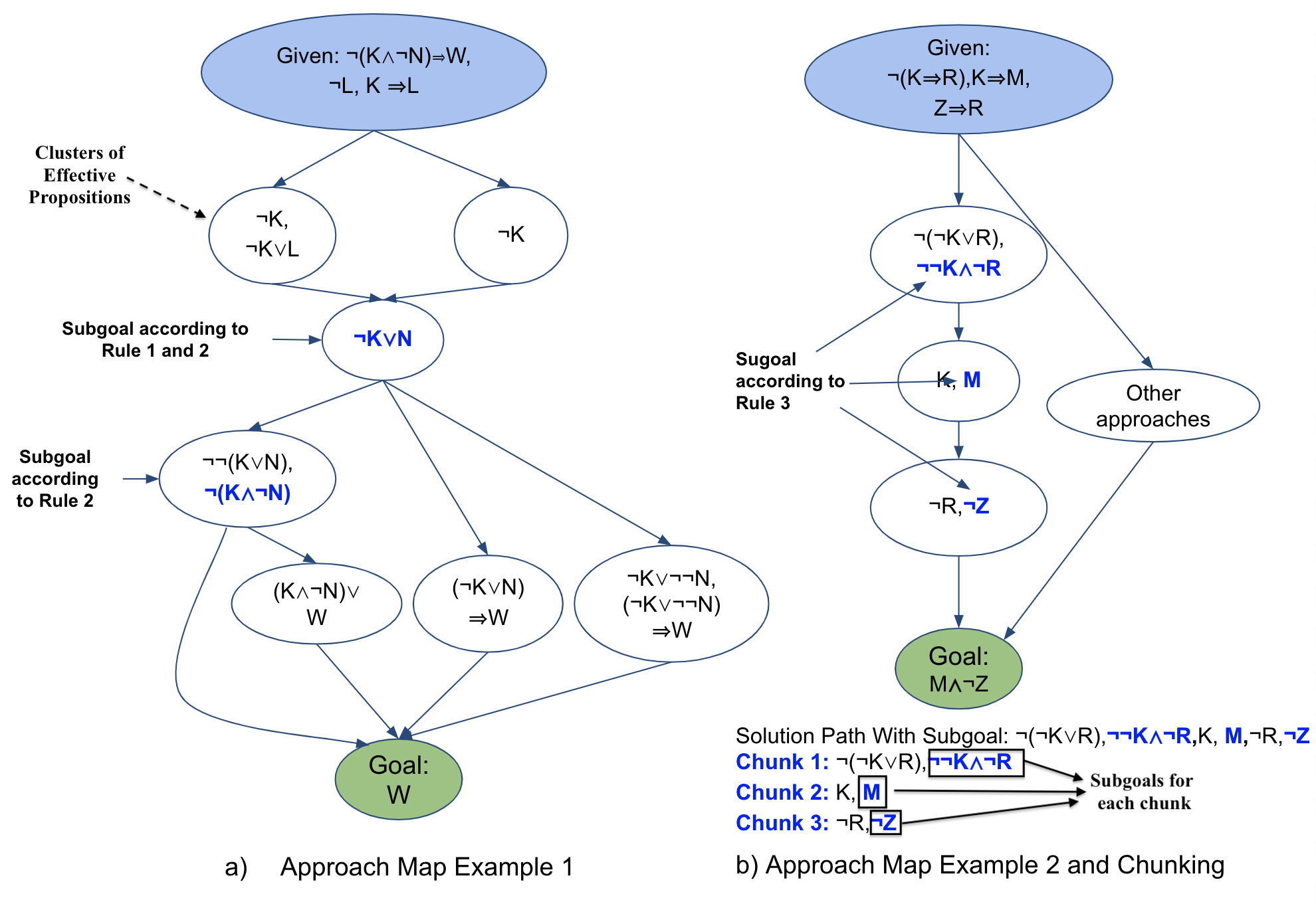
[sample approach maps are visualized in Figure 2]. Thus, this
representation is called an approach map [15]. Later, we used a
rule-based approach to extract chunks from the approach maps.
Extracting Chunks from Approach Maps: As discussed in Section
2, researchers [12, 19] have decomposed problem solutions
using constraints such that the decomposed sub-solutions can
be replaced with alternate solutions without causing any
problem. Based on this idea, we defined two rules to extract
pivot1
or subgoal propositions that are present in multiple approaches
and/or have multiple replaceable derivations within an approach
map (for example, \(\neg K\lor N\) in Figure 2a has two possible derivations
from the start state.). The rules to identify such pivots
are:
Rule 1: First proposition derived within a cluster where
multiple clusters merge is a pivot [\(\neg K\lor N\) in Figure 2a].
Rule 2: Last proposition derived within a cluster that generates
a fork is a pivot [\(\neg K\lor N\) and \(\neg (K\land \neg N)\) in Figure 2a].
Recall that an approach is a path from start to goal in an
approach map. And, being present in multiple paths or
approaches means that a proposition is possibly vital to the
proof and a subgoal in student approaches. Finally, we defined a
third rule to identify pivots in approaches that do not have a
common proposition with other approaches, i.e. they are simply
a linear chain of clusters of propositions[Figure 2b]. The third
rule is described below:
Rule 3: In a chain of clusters, the last derived node in each
cluster is a pivot [M or \(\neg Z\) in Figure 2b]. Note that in this rule, we
simply exploit the clusters identified by Girvan-Newman
algorithm to dismantle a complete solution into sub-solutions or
subgoals.
Finally, Using the three rules, we extracted the subgoals within the
most common student-solution approach for each DT logic-proof
problem while traversing its approach map from top to bottom.
We validated our pivot/subgoal- extraction process by
comparing our rule-based subgoals from approach maps against
expert-identified2
subgoals for 15 problems. And, our method was successful in
identifying all expert subgoals for those problems. After
validation, we used the subgoals to decompose the solution to
derive Chunks from them. An example of deriving chunks can
be found in Figure 2b. In the example, pivots/subgoals are
colored blue, and using the subgoals three chunks are extracted
from the complete solution. Note here that each chunk is
associated with a subgoal.
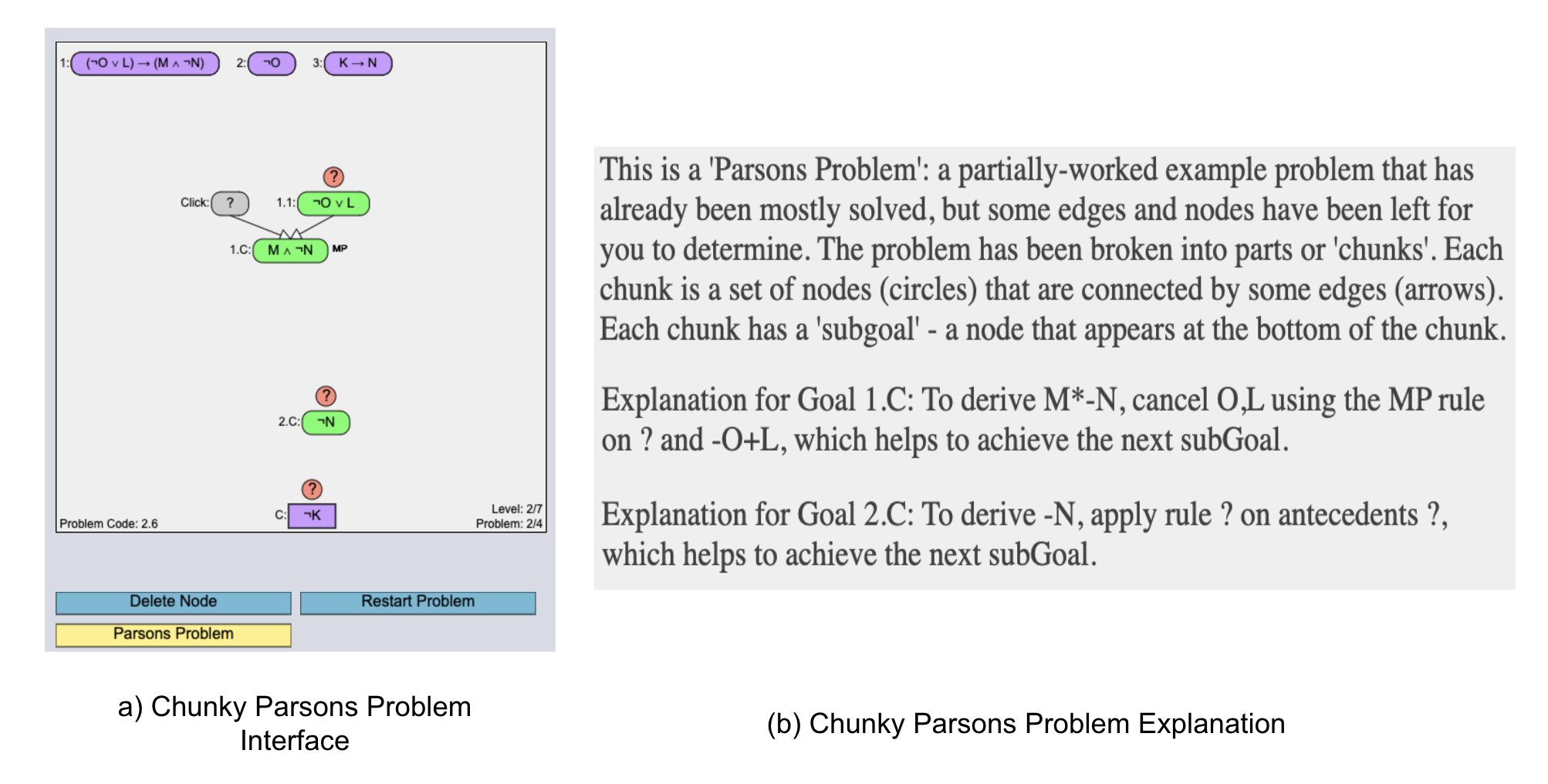
Explanations for Chunks: To accompany each of the chunks, we generated automated explanations using a script that explains the composition and purpose of the chunks. Before writing the script, a format for the chunk explanations was decided through discussion with an expert. Each explanation is written in natural language and tells what a chunk derives (i.e. the associated subgoal), how the subgoal is derived within the chunk, and why it is derived [Figure 3b]. The why part simply tells that each subgoal is necessary for the derivation of another subgoal or the final goal. Note that we paid close attention while crafting the explanation format so that it does not give away any information about the final solution beyond the visual representation of the chunks. Overall, the purpose of the explanations is just to highlight what the chunks represent (i.e. they are building blocks of a complete solution each deriving a subgoal).
3.2.1 Chunky Parsons Problem Interface
The Chunky Parsons Problem representation is shown in Figure 3a. In the presentation, the given premises and conclusion are presented as usual. And the chunks are presented as groups of connected propositions (or nodes) in a Parsons Problem fashion. The problem shown in Figure 3a has two chunks. All nodes within the chunks are connected to each other. However, the givens, the chunks, and the conclusion need to be connected by students to complete the proof. Each node within a chunk can be either justified (both antecedents present), partially justified (one of the antecedents missing as for \(M\land \neg N\)), or unjustified (all of the antecedents missing as for \(\neg O\lor L\) or \(\neg N\)). For justified and partially justified nodes, the associated logic rule is also shown. For example, in Figure 3a, \(M\land \neg N\) is labeled by MP, i.e. Modus Ponens is required for its derivation from the antecedents. In addition to the visual components, textual instructions containing chunk explanations [Figure 3b] were also provided to students who were assigned to a specific training condition (more details about training conditions in the next subsection). Note that the chunk or subgoal IDs (for example, 1.C, 2.C, etc. in the figure) are used to associate an explanation to a chunk and the IDs do not confirm the order of how the chunks should be connected to each other.
3.3 Experiment Design
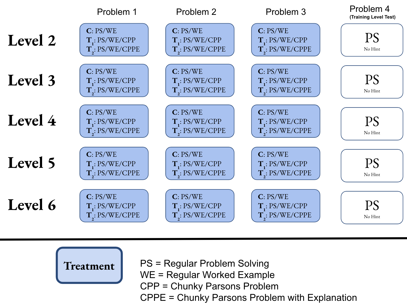
Using existing problem types within DT (PS and WE) and the
new problem types (CPP), we designed three training
conditions. The three training conditions are described
below:
Control (C): Students assigned to the Control (C) condition
received only PS or WE (selected randomly) during training.
Treatment 1 (\(T_1\)): Students assigned to this condition, may
receive CPP without explanation in addition to PS/WE
(selected randomly) during training.
Treatment 2 (\(T_2\)): Students assigned to this condition may
receive CPP with an explanation (i.e. CPPE) in addition to
PS/WE (selected randomly) during training.
Problem organization for each condition in the 5 DT training
levels is demonstrated in Figure 4. Note that the Control (C)
condition gives us a baseline for comparison between students
who received CPP or CPPE [i.e. \(T_1\)/\(T_2\) students]) and those who did
not receive CPP at all (i.e. C students). On the other hand, a
comparison between \(T_1\) and \(T_2\) helps to understand the impact
of the explicit explanation attached to each chunk in a
CPP.
System Deployment and Data Collection: We deployed DT with the three training conditions in an undergraduate logic course offered at a public research university in the Spring of 2022. Each participating student in that course was assigned to one of the three training conditions after they completed the pretest problems. Our training condition assignment algorithm ensures that the pretest scores of students in each of the training groups have a similar distribution. Finally, we had 50 students assigned to C, 50 students assigned to \(T_1\), and 45 students assigned to \(T_2\) who completed all 7 levels (pretest, all training levels, and the posttest level) of the tutor. We collected their pretest, training-level test, and posttest scores to compare performance/learning across the training groups. Additionally, we collected their solution traces to analyze differences in their proof construction approaches. Note that access to these data is restricted to IRB-authorized researchers. To answer our research questions, we carried out statistical and data-driven graph-mining-based analyses on the collected data that we report in the subsequent sections.
4. RESULTS
4.1 RQ1: Students’ Performance and Learning Gain
To understand the impact of each of our training conditions on students’ performance and learning, we analyzed students’ test score-based performance and normalized learning gain (NLG) after training. For these analyses, we focused on the training-level test problems (2.4-6.4) and the posttest problems (7.1-7.6) that students solved independently without any tutor help. We adopted a combination of regression and statistical analysis (Kruskal-Walis test with posthoc pairwise Mann-Whitney test with Bonferroni corrected \(\alpha \) = 0.0163) to compare the performance and learning gain across the three training conditions. These tests do not make an assumption about the data being perfectly normal. Since most of our collected data were skewed, these tests were considered suitable in this case. Note that there were no significant differences found in performance across the three groups in the pretest problems.
4.1.1 Test Score-based Performance
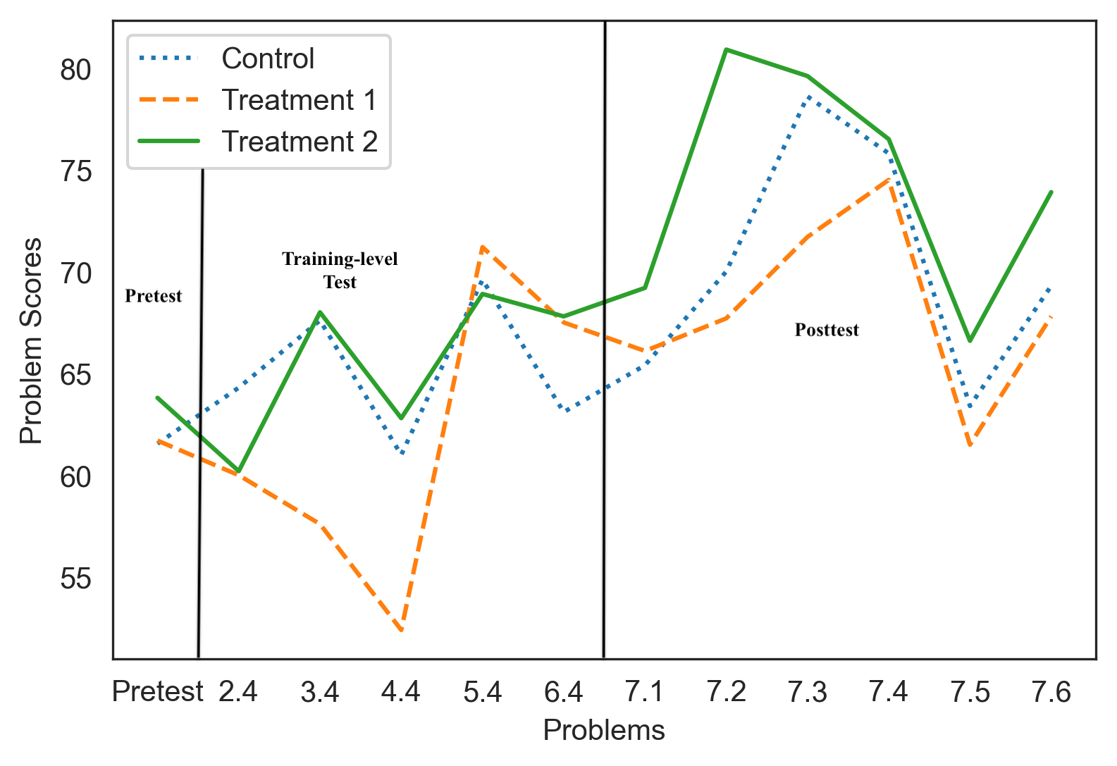
To identify the association between the training conditions and performance, we performed two mixed-effect regression analyses: one for the training-level test problems and one for the posttest problems. In each of these two analyses, problem IDs were defined as the random-effect variable (to eliminate the impact of differences across problems), training conditions were defined as the fixed-effect variable, and problem score was the dependent variable. The analysis for the training-level test problems [avg. training-level test scores(C, \(T_1\), \(T_2\)) = 65.1, 61.7, and 65.5] gave a p-value of 0.8 [p \(<\) 0.05 indicates significance] indicating that there was no significant association between training-level test performance and the training conditions. However, the analysis for the posttest problems [avg. posttest scores(C, \(T_1\), \(T_2\)) = 69.3, 68.2, and 73.5] gave a p-value of 0.06 demonstrating a marginally significant association between the training conditions and posttest performance. Also, the average posttest scores showed that \(T_2\) (who received CPPE) marginally outperformed the other two groups after 5 levels of training. To further investigate each training group’s posttest performance, we statistically compared scores across the three training groups in each of the independent posttest problem-solving instances (7.1-7.6). The trend in scores for these problems across the three training groups is shown in Figure 5. While analyzing the scores in the posttest problems, we observed that \(T_2\) had significantly higher scores than \(T_1\) and C in problems 7.1-7.3 [for 7.1, \(P_{MW}\)(\(T_2>T_1\))4 = 0.003 and \(P_{MW}\)(\(T_2>C\)) = 0.01, for 7.2, \(P_{MW}\)(\(T_2>T_1\)) = 0.02 and \(P_{MW}\)(\(T_2>C\)) = 0.01, and for 7.3, \(P_{MW}\)(\(T_2>T_1\)) = 0.03 (marginal) and \(P_{MW}\)(\(T_2>C\)) = 0.012] and higher average scores in problems 7.4-7.6. Note that posttest problems in DT are organized in increasing order of difficulty. Our analyses indicate that even though \(T_2\) could not significantly outperform the other two groups in the harder posttest problems(7.3-7.6), they performed comparatively better. This trend can be observed in the ‘Posttest’ fragment in Figure 5.
As shown in the figure, although \(T_2\) did not show a significantly higher average than the other two conditions in all problems, starting from problem 6.4, \(T_2\) students always had higher scores (shown by the solid green line) than the other two groups (shown by the dotted blue line and dashed orange line). Overall, from our regression and statistical analysis, we concluded that students’ posttest performance was associated with the training conditions, and the \(T_2\) training condition that involved CPPE was more helpful in improving students’ performance after training. However, \(T_2\) students showed evidence of improved performance around the end of training and in the posttest rather than showing gradual improvement over the period of training. A consistent pattern that indicates improved performance could not be identified for \(T_1\) students who received CPP without an explanation attached.
4.1.2 Normalized Learning Gain
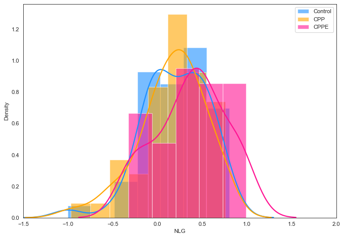
To identify the training condition that was most effective in promoting learning, we analyzed students’ normalized learning gain (NLG) across the three training conditions. NLG is defined as the ratio between how much the students learned and the maximum they could have learned between the period of pretest and posttest and is represented by the following equation: \begin {equation} NLG = (post - pre) / \sqrt {(100 - pre)} \end {equation} Note that NLG is normalized between -1 and 1. A negative NLG value represents that the posttest scores are lower than the pretest scores. Negative NLGs could occur if the students did not learn enough from training or if the posttest problems are significantly harder than the pretest problems. NLG for the three groups is shown in Table 1. We compared the NLGs across the three training groups using statistical tests. A Kruskal-Walis test demonstrated significant differences in the NLGs across the three training groups (statistic=5.8, p-val=0.05). As we carried out posthoc pairwise Mann-Whitney U tests with Bonferroni corrected \(\alpha \)=0.016, we observed \(T_2\) students had significantly higher NLGs than Control (C) (statistic=1283.0, p-val=0.01) and \(T_1\) (statistic=1235.0, pvalue=0.02) students. As we plotted the distribution of NLGs for the training groups in Figure 6, we observed that the distribution of NLGs for \(T_2\) is centered around positive (+) values, whereas the other two groups had tails on the negative (-) side. Also, as reported in Table 1, 80% of \(T_2\) students had a positive NLG, whereas the percentage for the other two groups are only 70% and 72% respectively. The results of this analysis on NLG indicate that training condition \(T_2\) (combination of CPPE with PS/WE) helped the students to learn better which moved their NLG above 0. Possibly, CPPE helped the students to perform comparatively well even in the harder problems (7.3 to 7.6) that could have caused negative NLG otherwise.
Group (n) | Pre | Post | NLG | %Student with(+) NLG |
|---|---|---|---|---|
| C (50) | 61.6(19.7) | 70.4(14.4) | 0.20(0.35) | 70% |
| T1(50) | 61.7(18.3) | 68.2(15.1) | 0.16(0.37) | 72% |
| T2(45) | 60.8(18.9) | 73.2(14.8) | 0.31(0.33) | 80% |
4.2 RQ2: Difficulties Associated with Solving Chunky Parsons Problems
The results from students’ performance analysis showed that CPP with explanations attached to chunks (i.e. CPPE) has the potential to improve students’ performance and learning gains. However, since it is a new type of problem-based training intervention, we acknowledged the necessity of analyzing its difficulty level in comparison to traditional training interventions like PS or WE. Since tutors like DT are often used by learners in the absence of a human tutor, our aim was to avoid increasing the training difficulty so that the students can persist and learn. Thus, we carried out a comparative analysis between the difficulty level of training CPP/CPPE and PS/WE problems. The difficulties associated with each problem type were measured by the average time that the students needed to solve them (i.e. the problem-solving time). Additionally, to guide future improvements so that the students are better supported during training with CPP/CPPE, we carried out an analysis to identify difficulties that could be associated with specific problem structures where students may need additional help to succeed. In the subsequent sections, we report the findings from the two analyses.
4.2.1 Comparative Difficulty Level of CPP/CPPE
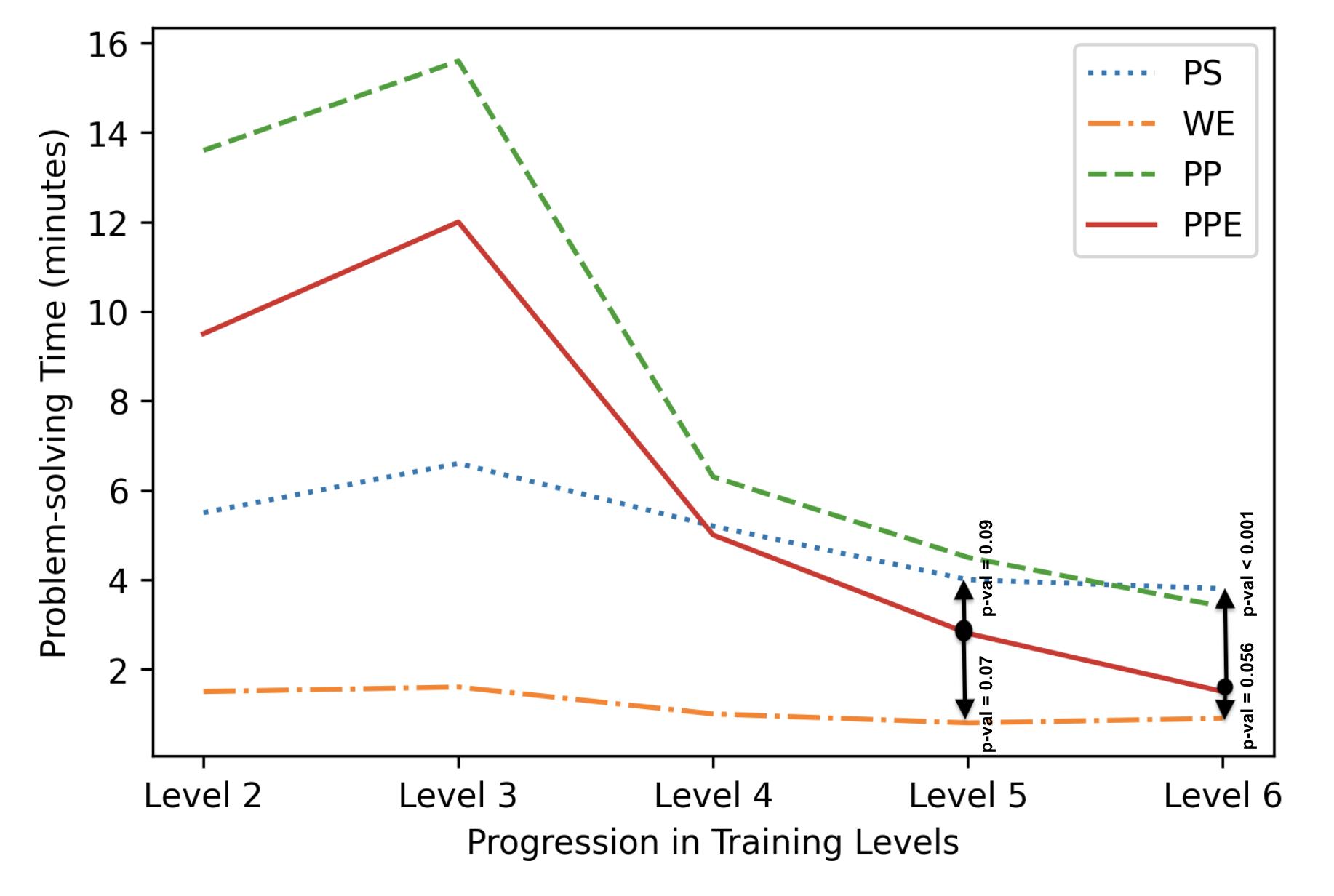
To understand the comparative difficulty level of CPP/CPPE, we compared the problem-solving times of CPP/CPPE against the problem-solving times of PS/WE using Mann-Whitney U tests. The plot representing problem-solving times for each of these problem types over the period of training is shown in Figure 7. Notice that in the first two training levels, students’ problem-solving time for CPP/CPPE was almost twice the problem-solving time of PS. This higher problem-solving time in the early training levels could be potentially associated with the additional time that the students needed to figure out how different components in the CPP/CPPE interface within DT work. However, as training progressed problem-solving time for CPP became more aligned with that of PS [notice the problem-solving times and comparative p-values at training levels 5 and 6 in Figure 7]. On the other hand, CPPE problem-solving times were marginally or significantly lower than that of PS at levels 5 and 6 respectively. Additionally, CPPE problem-solving times were only marginally higher than that of WEs in these two levels. These statistics indicate that the difficulty level of Chunky Parsons Problems (with/without explanation) lies in between the difficulty levels of PS/WE. However, with explanation, it can be a low-difficulty training task (difficulty level similar to WEs and lower than PS in terms of problem-solving time) that can help improve students’ learning gain.
4.2.2 Difficulties Associated with Specific Problem Structure
To identify difficulties associated with specific problem
structures, we calculated the average time students spent to
complete the proof of each chunk presented in a CPP/CPPE
(by connecting all nodes within a chunk to their correct
predecessor). We call this chunk-solving time. We identified 10
problems that contained chunks with chunk-solving time above
the 75th percentile (\(>\) 2.5 minutes) for at least \(10\%\) (\(>=\) 10 students) of
all \(T_1\) (CPP) and \(T_2\) (CPPE) students. To identify the difficulty
patterns in these problems, we carried out an exploratory
analysis of the structures of these problems and how the
students approached to solve the problem. For simplicity, while
explaining the problems associated with student difficulties, we
present only the abstract structure of the problems [Figure 8a,
b, and c]. In the abstract structure, we show how the chunks
need to be connected to solve the problem and rule categories
instead of the specific rules required to connect the chunks. We
grouped the available logic rules in DT into 3 categories: 1)
Transformation rules: transform the logic operator in between
variables or reorganize the variables in a proposition (Comm,
Assoc, DN, De Morgan, Impl, CP, Equiv, Dist), 2) Elimination:
remove one or more variables from proposition(s) (MP, MT, DS,
Simp, HS), 3) Combination: combines variables from two
propositions in one proposition (Add, Conj, CD). For the 10
problems, we identified three abstract problem structures
that are shown in Figure 8. Structure 1 was associated
with 6 problems. Structures 2 and 3 were associated with
2 problems each. Below we present our observations on
student difficulties (i.e. when and where in these structures
students spent more time) associated with each problem
structure:
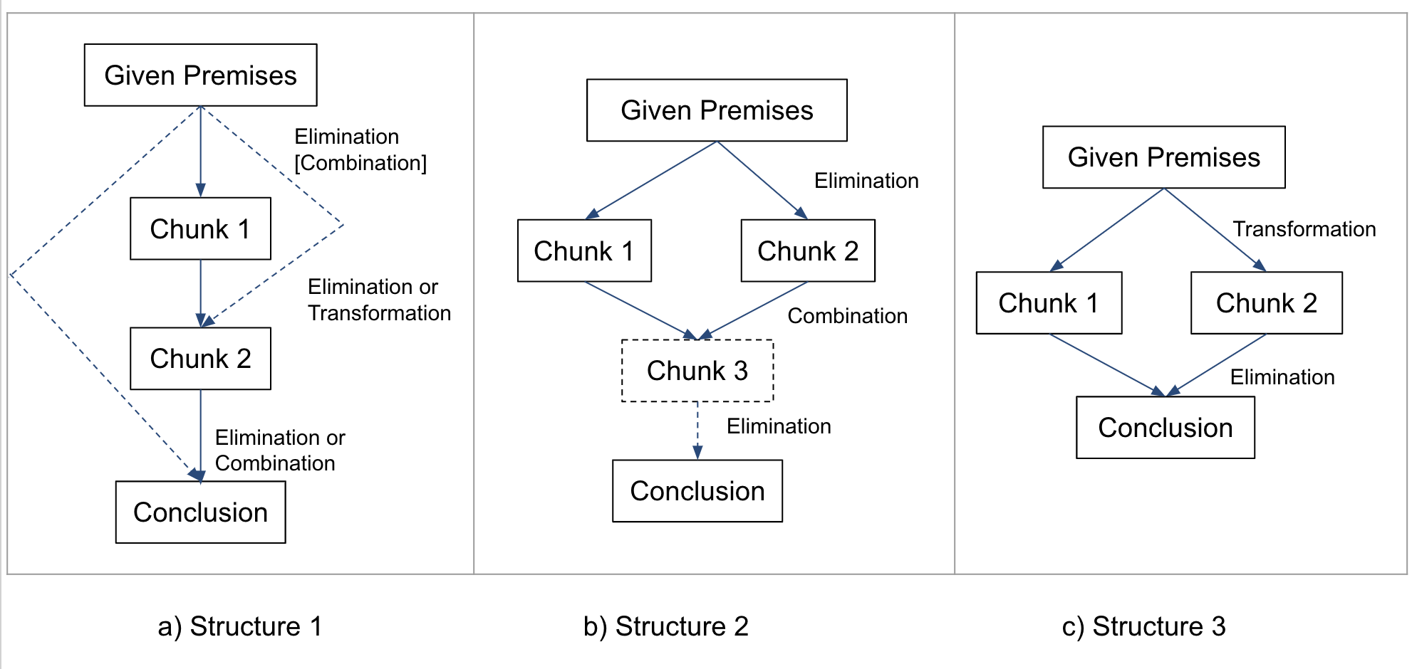
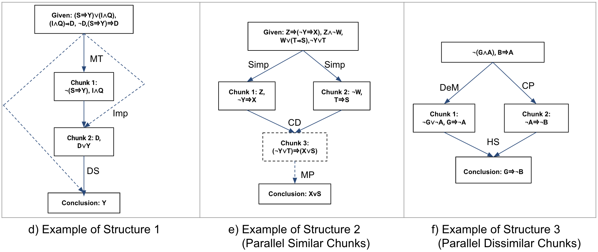
Structure 1: In structure 1 [Figure 8a], the chunks are
sequentially connected with different categories of rules. We
observed that within each of the six difficult problems with this
structure, there are almost no visual commonalities across
the chunks. An example problem with this structure is
shown in Figure 8d. In the figure, notice that each chunk
contains propositions composed of variables from almost
exclusive sets (Chunk 1 variables=S, I, Y, Q), Chunk 2
variables=D, Y), and also each chunk requires a different
rule.
In these 6 problems, we found 71 students (\(T_1\) = 39, \(T_2\) = 32) who
spent time above the 75th percentile to derive a chunk within at
least one of these problems. A total of 247 difficult instances
were found for these students solving problems with structure 1.
132 of those instances were associated with forward-directed
sequential derivation (i.e., the students completed the problem
in the following sequence, chunk 1 \(\rightarrow \) chunk 2 \(\rightarrow \) conclusion), 11
were associated with backward-directed sequential derivation
(i.e., the students completed the problem in the following
sequence, conclusion \(\rightarrow \) chunk 2 \(\rightarrow \) chunk 1), and 104 instances were
associated with random derivation where students moved
from chunk to chunk without demonstrating a strategical
pattern.
Overall, after the analysis of the structure of the 6 problems and
student approaches to solving the problems (forward, backward,
or random), we could not associate a specific approach with the
chunk-solving difficulty. Rather, we concluded that the difficulties
could be associated with the diversity in rules/variables across
chunks within the problems that possibly increased cognitive
load5
introducing difficulties for students.
Structure 2: In structure 2 [Figure 8b], two parallel chunks
(chunk 1 and chunk 2) with very similar derivations are
combined to derive the conclusion or a third chunk (chunk 3)
that later helps to derive the conclusion. We found 2 difficult
problems associated with structure 2. An example problem for
this structure is shown in Figure 8e.
We identified 40 students (18 \(T_1\) students, 22 \(T_2\) students) who
at least had one difficult instance (i.e. spent above 75th
percentile of time) while solving one of the problems associated
with this structure. 50 difficult instances [16 associated
with forward-directed sequential derivation, 1 associated
with backward-directed sequential derivation, and 33 with
random derivation] were found for these students while
solving one of these 2 problems. We observed that the
students spent more time on either chunk 1 (31 instances)
or chunk 2 (19 instances) depending on whichever they
attempted to complete first. We also observed that they spent
average or below-average time while deriving the rest of the
chunks.
These observations indicate that the students were able to
identify similarities across the chunks within a problem. Thus,
although they spent more time on the first chunk, after figuring
out the derivation of the first chunk, they needed less time to
derive the rest.
Structure 3: Structure 2 and structure 3 [Figure 8c] are
visually very similar. However, the main difference is that the
derivations of chunk 1 and chunk 2 within structure 3 have no
similarities (an example problem is shown in Figure 8f).
We found 2 difficult problems associated with structure
3.
33 students were identified (19 \(T_1\) students, 14 \(T_2\) students) who
had at least one difficult derivation (i.e. spent above 75th
percentile of time) while solving one of the problems associated
with this structure. 45 difficult instances [28 associated
with FW-directed sequential derivation, 13 associated with
BW-directed derivation, and 4 with random derivation]
were found for these students while solving one of these 2
problems. And, we observed that in most of the cases, students
spent higher time on both chunk 1 and chunk 2 (total 35
instances).
Overall, our observations indicate that difficulties mostly
occurred when chunks within a problem were very dissimilar (in
Structure 1 and Structure 3). On the other hand, if there are
similar chunks within a problem, after deriving one chunk, the
students figured out the derivation of other similar chunks very
quickly.
4.2.3 Learning Efficiency and Correlation Test between NLG and Training Time
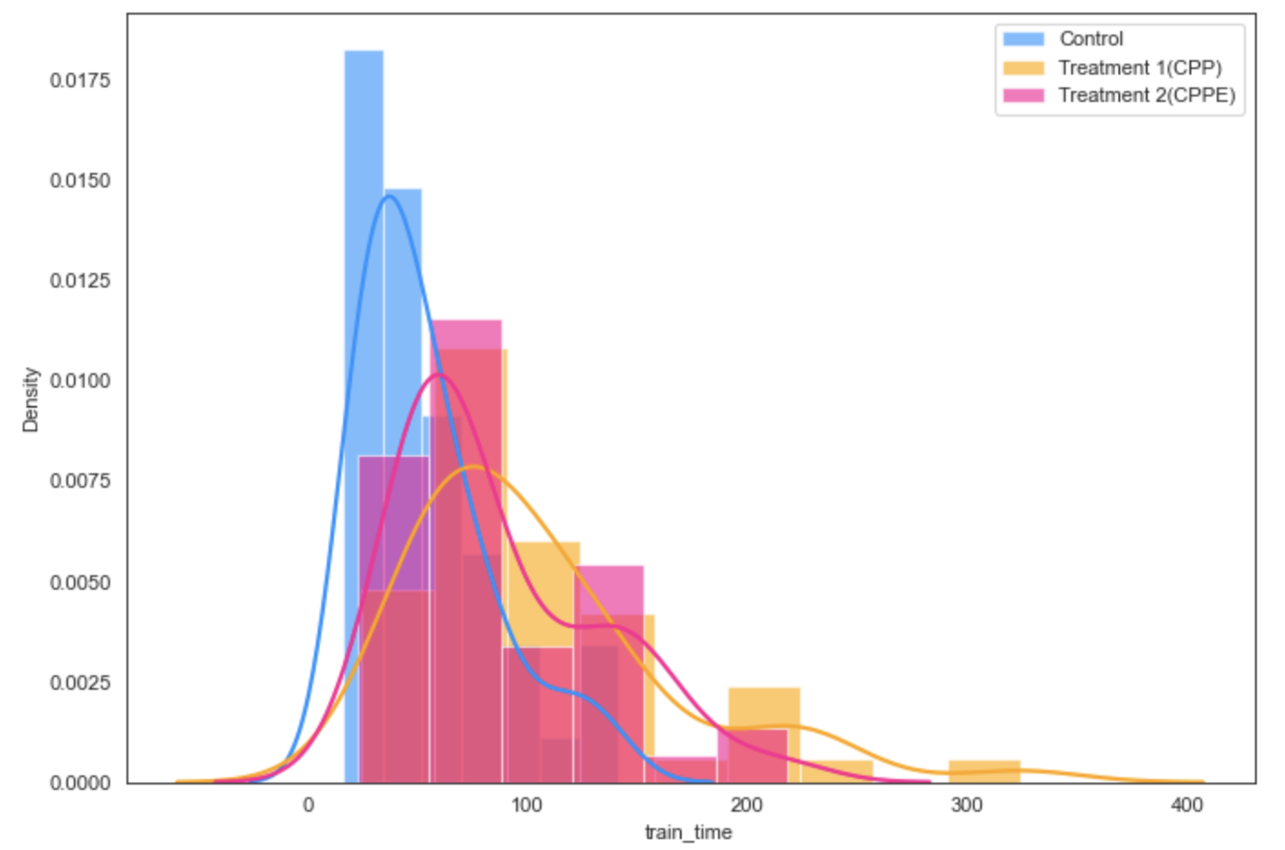
Overall, the training time for \(T_1\) (this group received CPP
without any explanation) and \(T_2\) (this group received CPP with
explanations) was higher than the control group [Control (C):
66.4(35.3) minutes, \(T_1\) (CPP): 89.7 (60.7) minutes, \(T_2\) (CPPE): 81.8
( 46.0) minutes]. The skewed distribution of training times
across the three training conditions is visualized in Appendix
B, Figure 12.
Since the training times were higher for the treatment groups,
we calculated the learning efficiency (NLG/Training Time) for
each group. However, we did not find any difference in learning
efficiency across the groups [Control (C): 0.007( 0.011), \(T_1\) (CPP):
0.003( 0.005), \(T_2\) (CPPE): 0.004(0.009). Kruskel-Wallis Test:
(statistic=2.84, p-value=0.24); Pairwise post-hoc Mann
Whitney U Tests: (C, \(T_1\))=(statistic= 986.0, p-value=0.30), (C,
\(T_2\))=(statistic=1020.0, p-value = 0.11), (\(T_1\), \(T_2\))=(statistic=1231.0,
p-value=0.43)]. We also did not find any significant correlation
between NLG and training times [Control (C): coefficient =
-0.09, p-value = 0.32; \(T_1\) (CPP): coefficient = -0.21, p-value =
0.96; \(T_2\) (CPPE): coefficient = 0.01, p-value = 0.43]. Therefore, it
is unclear whether or not the differences in NLG across the
training conditions occurred due to differences in training
times.
5. RQ3: STUDENTS’ CHUNKING BEHAVIOR
CPP and CPPEs were incorporated within DT training levels to
demonstrate chunking (i.e. decomposed problem solutions),
engage students in the process (by having them recompose
complete solutions from chunks), and motivate them to adopt
chunking (i.e. decomposition-recomposition (PDR)) to reduce
difficulties while solving new problems. To investigate if
students successfully captured the notion of chunking while
solving CPP/CPPE and if they tried to form chunks when
solving problems independently (which we refer to as chunking
behavior), we adopted a data-driven approach. From log data
collected within DT, we tried to infer if the students showed
chunking/PDR behavior and how the behavior was associated
with their performance.
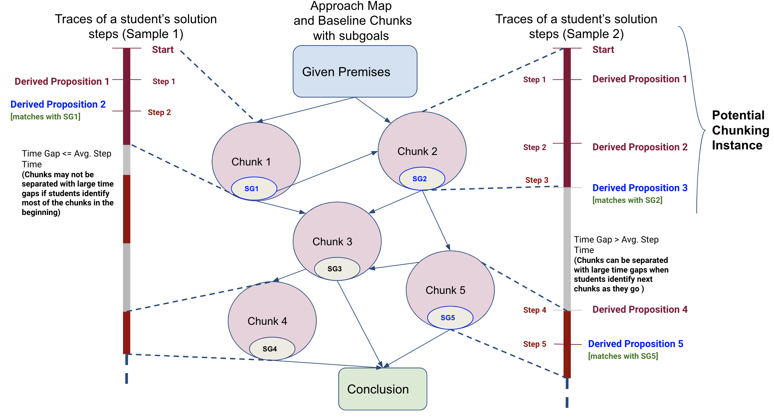
Method to Identify Chunking Behavior: We analyzed students’
chunking behavior in the posttest problems that they solved
independently [7.1-7.6]. To do so, first, we derived baseline
chunks from historical student solutions to these problems. For
problems 7.1-7.6, using the method described in Section 3.2, we
generated approach maps using historical data collected in DT
to capture previous students’ solutions and identified baseline
chunks in those solutions. The baseline chunks answer ’What to
look for in the solutions of the students participating in this
study’. Next, to confirm the presence of the baseline chunks or
chunking/PDR behavior in a student’s proof construction
attempt, we sequentially scanned through the student’s
steps while constructing a proof and identified consecutive
steps as chunking when the step sequence has the following
characteristics:
1. The propositions derived in the step sequence overlaps with
propositions and subgoal associated with only one of the
baseline chunks [we applied the ‘Intersection’ set operation to
find an overlap].
2. The step sequence may or may not be separated from the rest
of the steps by a time gap above the average step time (the time
spent on a single step) of 1.6 minutes. The two cases of
separation by time gaps are shown in Sample 1 and Sample 2 in
Figure 9.
The process of identifying chunking in a student solution
attempt is further illustrated in Figure 9.
Learning and Chunking Behavior: Following prior research [9, 25],
to validate our method to identify chunking behavior, we
sought to explain students’ learning gain that reflects their
problem-solving skills through derivation efficiency in the
chunking instances detected using our method.
We hypothesized that a higher number of treatment group
students (who received CPP/CPPE) will have chunking
instances in their solutions of posttest problems than the
control(C) group students. However, we identified that most of
the students (121 out of the 145 students) regardless of their
training conditions had baseline chunks present in their
solutions. Only 24 students (C=8,\(T_1\)=9,\(T_2\)=6) never showed any
identifiable chunking behavior. This indicates that students
might have a natural tendency to identify sub-problems and
construct logic proofs in chunks. Whereas the presence of some
chunking instances is desirable, too many chunks in a problem
solution do not represent better performance and more learning.
Deep Thought proofs are usually 7-15 steps long and an ideal
solution for each problem mostly contains 2-3 chunks. Since the
Deep Thought problem score which impacts NLG is designed
as a function of time, step counts, and rule application
accuracy, to achieve higher scores and NLG, students need to
demonstrate only correct baseline chunks within their solutions
and each of those chunks needs to be derived efficiently
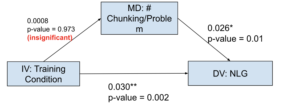
with less time and fewer steps. This fact was validated by
a mediation analysis. In the analysis, we used training
condition as the independent variable (IV), NLG as the
dependent variable (DV), and average # chunks/problem as the
mediator (MD). The analysis gave an insignificant p-value
[Appendix B, Figure 14] indicating that the impact of the
training treatments on learning or NLG is not mediated by
the amount of chunking present in students’ logic-proof
solutions.
Thus, in subsequent analyses, instead of focusing on the number
of chunks present in student solutions, we focused only on
students’ efficiency in deriving the baseline chunks. We
calculated efficiency in terms of time spent on deriving different
chunks and # of steps within the chunks. We also analyzed
NLGs across different pretest score groups to understand the
impact of CPP/CPPEs on students with different levels of prior
knowledge.
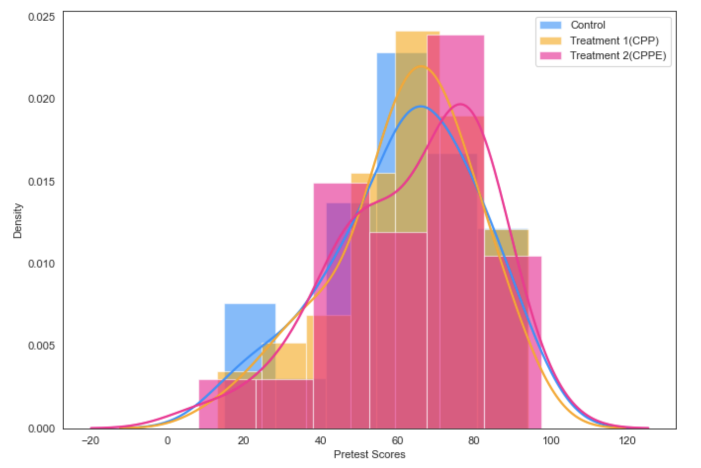
Moderation Analysis on Different Pretest Score Groups: Prior
studies showed that both worked examples and Parsons
problems may have a different impact on students based on
their prior knowledge or skill level [34, 17]. We carried
out a moderation analysis to understand how NLG and
chunking behavior and efficiency varied across different pretest
score groups and training conditions. The pretest score
distribution is visualized in Appendix B, Figure 13. We
classified students based on their pretest scores (low, medium,
and high) and used this classification as the moderator
in our analysis. Within this classification, we considered
training condition as the independent variable. For each
pretest score group and training group, we analyzed 4
dependent variables: average # chunks/problem, average chunk
time, avg. chunk step count, and the NLG. Table 2 shows
the groupings and values for the dependent variables. To
compare the dependent variables across pretest score groups
and training conditions, we carried out Kruskal Wallis
test and pairwise posthoc Mann Whitney U tests with
Bonferroni correction (corrected \(\alpha =\) 0.05/3 or 0.016). Note that
a total of 36 tests(3 pretest score groups, 4 dependent
variables, and 3 pairwise tests for each group and dependent
variable) were carried out to compare the metrics presented in
Table 2. Thus, a more conservative Bonferroni correction
could be carried out to eliminate false positives. However,
to not introduce many false negatives while eliminating
false positives, we decided the level of correction based
on the number of unique pairwise tests each datapoint
participated in [6] rather than on the number of related
tests (for example, the 9 tests on NLG across the pretest
scores groups though independent could be considered
related and a more conservative correction could be carried
out). We explain the results for each pretest score group
below:
Low Pretest Scorers: We considered students with pretest scores
below the 25th percentile as low scorers. In this group, we
observed that \(T_2\) who received CPPE had significantly higher and
less negative NLGs than the other two training conditions [\(p_{KW} < 0.001\), \(p_{MW}(T_2 > C)\) =
0.011, \(p_{MW}(T_2 > T_1) <\) 0.001]. We also observed that \(T_2\) students with low pretest
scores had lower average chunk time and significantly lower step
counts per chunk [\(p_{KW} < 0.03\), \(p_{MW}(T_2 < C)\) = 0.004, \(p_{MW}(T_2 < T_1) <\) 0.014]. Overall, \(T_2\) students with low
pretest scores demonstrated comparatively more efficient
chunking (in terms of less time and step counts) and higher
NLG. However, a difference in the number of chunks per
problem was not found across the training conditions as
expected.
Medium Scorers: Students with pretest scores between
25th-75th percentile were identified as the medium scorers.
Within this group, we observed that the \(T_2\) condition again
showed significantly or marginally higher NLG than the other
two training conditions [\(p_{KW} < 0.001\), \(p_{MW}(T_2 > C)\) = 0.002, \(p_{MW}(T_2 > T_1) <\) 0.021]. We observed
differences in the averages of chunk time across the three
training conditions, however, a significant difference was not
found in chunk count, time, or step counts.
High Scorers: We did not observe any significant differences in
NLG across the three training conditions for students with
high pretest scores (above 75th percentile). However, we
observed that \(T_1\) and \(T_2\) students in the high pretest score group
demonstrated comparatively more chunking (in the range of 3-4
chunks per problem) in posttest than the control (C) group (in
the range of 2-3 chunks per problem).
Overall, the results of the moderation analysis indicate that \(T_2\)
students with low and medium pretest scores achieved
significantly higher NLGs than students from the other two
training conditions with similar levels of prior knowledge. There
were no significant differences in the amount of chunking per
problem across the training conditions. However, we observed
differences in the chunking efficiency where \(T_2\) had lower chunk
derivation times and fewer steps within chunks in some cases.
Thus, next, we analyze and present the chunking efficiency
across the three training conditions on different posttest
problems in further detail.
Chunk Derivation Efficiency: We compared the chunk
derivation efficiency of the students across the three training
conditions who had identifiable chunks in their solutions.
Toward that, we analyzed two metrics for the baseline chunks
identified in student solutions to the posttest problems: 1)
Time to derive a chunk (shorter chunk derivation time
[CTime] indicates students figured out ‘how to derive
the chunk’ quickly), 2) unnecessary proposition count
[UProp]6
(fewer unnecessary propositions indicate students correctly
identified ‘what to derive within the chunk’). Lower values
for these two metrics indicate higher chunk derivation
efficiency.
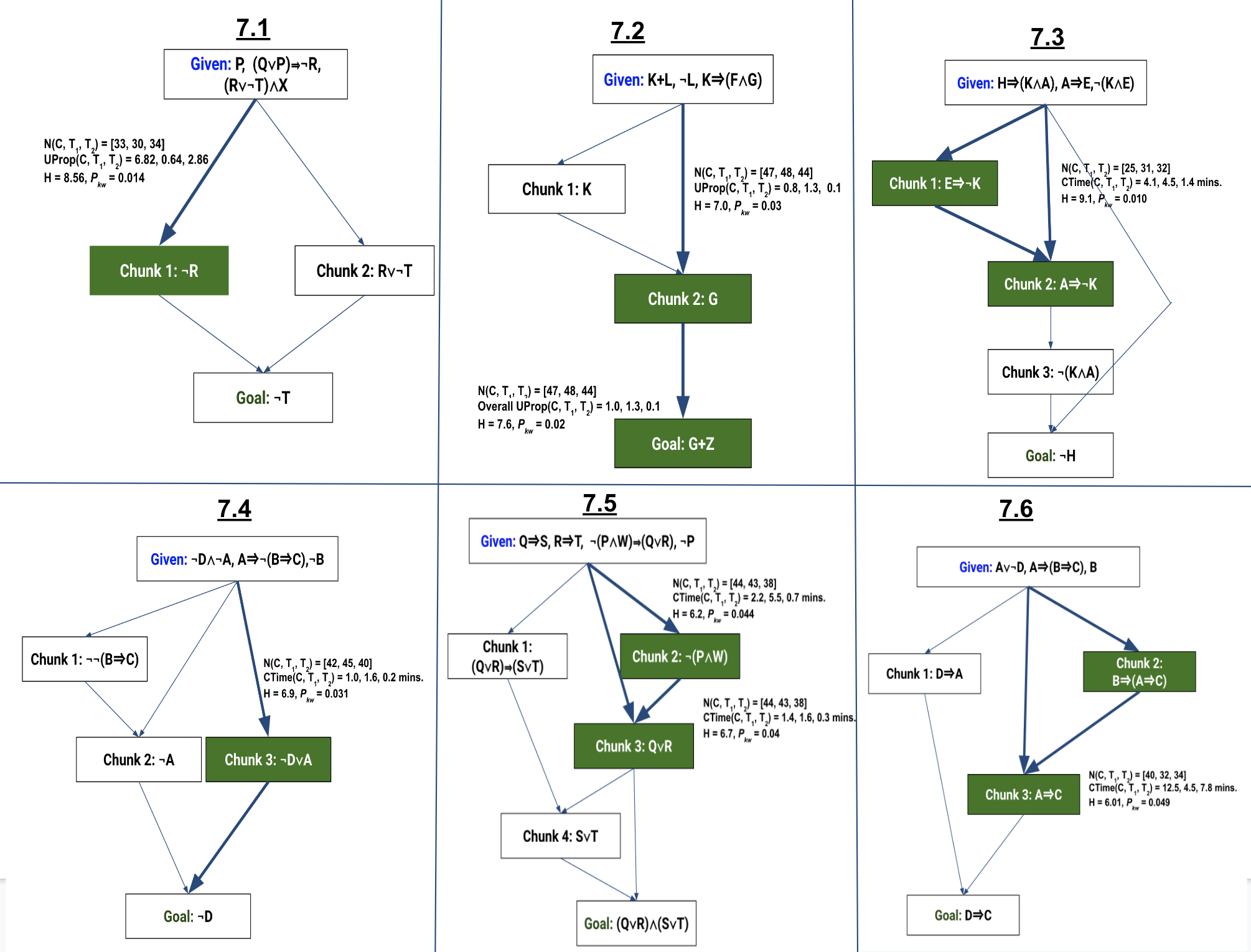
In Figure 10, we show the chunks commonly found in students’
proof for each of the posttest problems. For simplicity,
for each of the chunks, we only show what subgoal the
chunk derives. To identify significant differences in the
derivation efficiency of these chunks (in terms of CTime or
UProp) across the three training conditions, we carried
out Kruskal-Wallis tests. The chunks for which there is a
significant difference in derivation efficiency across the training
conditions in terms of at least one of UProp or CTime are
marked with thicker edges and green nodes in the figure. The
results of the statistical tests are shown along the thicker
edges. We observed that the significant differences were
found mostly for non-trivial chunks, i.e. chunks that involve
several proposition derivations. For example, there are two
chunks in the solution of 7.1: the first chunk derives \(\neg R\) which
requires multiple steps (i.e. non-trivial), and the second
chunk derives \(R\lor \neg T\) which can be derived after a Simplification
rule application on the given premise \((R\lor \neg T)\land X\) (trivial derivation).
We found significant differences only in the derivation
efficiency of chunk 1 (the non-trivial chunk). To identify the
training condition that was the most efficient in deriving the
green chunks in Figure 10, we carried out posthoc pairwise
Mann-Whitney U tests [for the pairs (C, \(T_1\)), (C, \(T_2\)), and (\(T_1\), \(T_2\))]
with Bonferroni correction (corrected \(\alpha \)=0.016) comparing
UProb and CTime. The results of the tests are shown in
Table 3. As shown in the table, in most of the cases, \(T_2\) is the
most efficient group in deriving the chunks, i.e. the tests
for the hypotheses ‘\(T_2 < C\)’ and ‘\(T_2 < T_1\)’ in terms of UProp/CTime
gave p-value \(<\) 0.016. Overall, these results indicate that
although most students naturally derived chunks, \(T_2\) students
achieved higher efficiency in deriving non-trivial chunks.
| Moderator | Independent Variable (IV) | Dependent Variables (DV)
| |||
|---|---|---|---|---|---|
Pretest Quantile | Training Condition | Avg. # chunks/ prob. | NLG | Avg. Chunk Time (minutes) | Avg. Chunk Step Count |
Low Scorers (\(<\) 25th percentile) N = 35 | Control(n=12) | 2.02(3.25) | -0.20(0.35) | 3.42(1.45) | 2.01(0.81) |
| \(T_1\)-CPP(n=12) | 2.47(3.62) | -0.40(0.39) | 2.78(3.80) | 2.06(1.03) | |
| \(T_2\)-CPPE(n=11) | 2.19(3.54) | -0.07(0.22)* | 2.21(3.26) | 1.94(0.90)* | |
Medium Scorers (25th-75th percentile) N = 75 | Control(n=25) | 2.51(3.98) | 0.34(0.23) | 2.88(4.51) | 2.25(1.38) |
| \(T_1\)-CPP(n=26) | 2.58(3.96) | 0.35(0.25) | 3.03(5.15) | 2.05(1.08) | |
| \(T_2\)-CPPE(n=23) | 2.26(3.60) | 0.48(0.22)* | 2.45(3.90) | 2.14(1.14) | |
High Scorers (\(>\) 75th percentile) N = 35 | Control(n=13) | 2.92(3.72) | 0.30(0.17) | 3.09(4.22) | 2.45(1.34) |
| \(T_1\)-CPP(n=11) | 3.50(4.5) | 0.32(0.13) | 4.03(5.64) | 2.16(0.89) | |
| \(T_2\)-CPPE(n=11) | 3.13(3.96) | 0.33(0.17) | 2.94(3.47) | 2.31(1.26) | |
| Problem | Chunk | Metric | Pairwise Mann- Whitney U Test |
|---|---|---|---|
| 7.1 | Chunk 1 | UProp | p(T1 p(T2 |
| 7.2 | Chunk 2 | UProp | p(T2 p(T2 |
| 7.3 | Chunk 1 + Chunk 2 | CTime | p(T2 p(T2 |
| 7.4 | Chunk 3 | CTime | p(T2 p(T2 |
| 7.5 | Chunk 2 + Chunk 3 | CTime | p(T2 p(T2 |
| 7.6 | Chunk 2 + Chunk 3 | CTime | p(T1 p(T2 |
6. DISCUSSION
Overall, our analysis showed that Chunky Parsons problem
could be a low-difficulty training intervention, specifically when
presented with an explanation hinting at what the chunks
mean and how they contribute to the complete solution.
However, while being a low-difficulty training intervention,
it has the potential to improve students’ learning gain
and problem-solving skills, specifically chunking skills. We
observed that most students formed some chunks during proof
construction. However, students from all training conditions
were not equally efficient in chunking. Our statistical tests
showed that \(T_2\) (who received CPP with an explanation attached
to chunks) derived non-trivial chunks with higher efficiency.
However, this efficiency often was not observed for all chunks
within a problem. Another limitation of CPP/CPPEs is the
difficulties associated with it when students first encounter
CPP/CPPE in early training levels or when the chunks within a
CPP/CPPE are very diverse. Thus, we recommend providing
additional guidance or tutor help in these scenarios to ensure a
better student experience while solving and learning through
CPP/CPPE. Nevertheless, our analyses have established that
Chunky Parsons Problems with explanations can be an
effective problem-based training intervention to improve
students’ Chunking skills (i.e. problem decomposition into
chunks and recomposing them to construct a complete
solution).
Also, our data-driven method to derive subgoals can be
adopted for any structured problem-solving domain as
long as each step during problem solving can be presented
as a state transition. For example, in a math-expression
evaluation problem, a state can be the set of all evaluated
parts of the equation at a particular moment. A step or an
action (for example, applying a math operator) changes the
problem state. Once the state transitions or interaction is
defined within a domain, generating the approach maps and
extracting subgoals from them can be carried out generically
(graph construction, applying clustering, and simplifying the
graph in approach maps). Similarly, the chunking efficiency
evaluation method can be adopted in other domains, as
long as each point in the students’ sequential problem
solution traces can be presented as a state from a finite state
space.
7. CONCLUSION AND FUTURE WORK
The contributions of this paper are 1) the demonstration of a
data-driven graph-mining-based method to decompose
problem solutions into expert-level chunks, 2) the design of a
problem-based training intervention called Chunky Parsons
Problem to be used within an intelligent tutor to teach students
the concept of structural decomposition-recomposition (or
Chunking) of problems, 3) an evaluation of the impact of
Chunky Parsons Problem on learning and students’ chunking
skills, and 4) a mechanism to identify Chunking in students’
solution traces using historical baseline chunks. As discussed
earlier, our data-driven methods to derive Chunky Parsons Problem and to identify Chunking in student solution traces can
be adapted for any domain where problem solving is structured
and the states and transitions of students during problem
solving can be defined definitely. Likewise, Chunky Parsons
Problem can be adapted for any problem-based tutor within
such domains.
However, this study has several limitations. First, the design
decisions for Chunky Parsons Problems (CPPs) and their
explanations were made based on prior literature, without any
user studies to validate them. Second, while we validated chunks
found in participants’ solutions, our data-driven evaluation
method may not be able to detect new chunks that were not
previously seen in prior student data. Also, the outcomes of this
study are dependent on how we defined different data-driven
metrics (for example, difficulty or efficiency). Third, although
our evaluation can identify the impact of interventions, it
cannot validate the source of the impact. Thus, future user
studies involving interviews or talk-aloud protocols could help
address these three issues and validate the findings on the
usability and impact of Chunky Parsons Problem. Finally, our
study focused only on logic-proof problems and should be
replicated in other domains to understand the generalizability of
the findings.
8. ACKNOWLEDGMENTS
The work is supported by NSF grant 2013502.
9. REFERENCES
- M. Abdelshiheed, J. W. Hostetter, P. Shabrina, T. Barnes, and M. Chi. The power of nudging: Exploring three interventions for metacognitive skills instruction across intelligent tutoring systems. In Proceedings of the 44th annual conference of the cognitive science society, pages 541–548, 2022.
- M. Abdelshiheed, J. W. Hostetter, X. Yang, T. Barnes, and M. Chi. Mixing backward-with forward-chaining for metacognitive skill acquisition and transfer. In Artificial Intelligence in Education, pages 546–552. Springer, 2022.
- M. Abdelshiheed, G. Zhou, M. Maniktala, T. Barnes, and M. Chi. Metacognition and motivation: The role of time-awareness in preparation for future learning. In Proceedings of the 42nd annual conference of the cognitive science society, pages 945–951, 2020.
- T. Barnes and J. Stamper. Toward the extraction of production rules for solving logic proofs. In AIED07, 13th International Conference on Artificial Intelligence in Education, Educational Data Mining Workshop, pages 11–20, 2007.
- D. Barr, J. Harrison, and L. Conery. Computational thinking: A digital age skill for everyone. Learning & Leading with Technology, 38(6):20–23, 2011.
- J. M. Bland and D. G. Altman. Multiple significance tests: the bonferroni method. Bmj, 310(6973):170, 1995.
- R. Catrambone. Aiding subgoal learning: Effects on transfer. Journal of educational psychology, 87(1):5, 1995.
- R. Catrambone. The subgoal learning model: Creating better examples so that students can solve novel problems. Journal of experimental psychology: General, 127(4):355, 1998.
- C. Charitsis, C. Piech, and J. C. Mitchell. Using nlp to quantify program decomposition in cs1. In Proceedings of the Ninth ACM Conference on Learning@ Scale, pages 113–120, 2022.
- O. Chen, S. Kalyuga, and J. Sweller. The worked example effect, the generation effect, and element interactivity. Journal of Educational Psychology, 107(3):689, 2015.
- T. J. Cortina. An introduction to computer science for non-majors using principles of computation. Acm sigcse bulletin, 39(1):218–222, 2007.
- G. B. Dantzig and P. Wolfe. Decomposition principle for linear programs. Operations research, 8(1):101–111, 1960.
- P. J. Denning. The profession of it beyond computational thinking. Communications of the ACM, 52(6):28–30, 2009.
- P. Denny, A. Luxton-Reilly, and B. Simon. Evaluating a new exam question: Parsons problems. In Proceedings of the fourth international workshop on computing education research, pages 113–124, 2008.
- M. Eagle and T. Barnes. Exploring differences in problem solving with data-driven approach maps. In Educational data mining 2014, 2014.
- M. Eagle, D. Hicks, and T. Barnes. Interaction network estimation: Predicting problem-solving diversity in interactive environments. International Educational Data Mining Society, 2015.
- B. J. Ericson, J. D. Foley, and J. Rick. Evaluating the efficiency and effectiveness of adaptive parsons problems. In Proceedings of the 2018 ACM Conference on International Computing Education Research, pages 60–68, 2018.
- G. V. F. Fabic, A. Mitrovic, and K. Neshatian. Evaluation of parsons problems with menu-based self-explanation prompts in a mobile python tutor. International Journal of Artificial Intelligence in Education, 29(4):507–535, 2019.
- K. B. Gallagher and J. R. Lyle. Using program slicing in software maintenance. IEEE transactions on software engineering, 17(8):751–761, 1991.
- J. S. Gero and T. Song. The decomposition/recomposition design behavior of student and professional engineers. In 2017 ASEE Annual Conference & Exposition, 2017.
- M. Girvan and M. E. Newman. Community structure in social and biological networks. Proceedings of the national academy of sciences, 99(12):7821–7826, 2002.
- S. Grover and R. Pea. Computational thinking in k–12: A review of the state of the field. Educational researcher, 42(1):38–43, 2013.
- M. Guzdial. Education paving the way for computational thinking. Communications of the ACM, 51(8):25–27, 2008.
- V. Karavirta, J. Helminen, and P. Ihantola. A mobile learning application for parsons problems with automatic feedback. In Proceedings of the 12th koli calling international conference on computing education research, pages 11–18, 2012.
- J. S. Kinnebrew, K. M. Loretz, and G. Biswas. A contextualized, differential sequence mining method to derive students’ learning behavior patterns. Journal of Educational Data Mining, 5(1):190–219, 2013.
- K. Kwon and J. Cheon. Exploring problem decomposition and program development through block-based programs. International Journal of Computer Science Education in Schools, 3(1):n1, 2019.
- L. A. Liikkanen and M. Perttula. Exploring problem decomposition in conceptual design among novice designers. Design studies, 30(1):38–59, 2009.
- M. Maniktala and T. Barnes. Deep thought: An intelligent logic tutor for discrete math. In Proceedings of the 51st ACM Technical Symposium on Computer Science Education, pages 1418–1418, 2020.
- L. E. Margulieux, M. Guzdial, and R. Catrambone. Subgoal-labeled instructional material improves performance and transfer in learning to develop mobile applications. In Proceedings of the ninth annual international conference on International computing education research, pages 71–78, 2012.
- J. J. McConnell and D. T. Burhans. The evolution of cs1 textbooks. In 32nd Annual Frontiers in Education, volume 1, pages T4G–T4G. IEEE, 2002.
- B. B. Morrison, L. E. Margulieux, B. Ericson, and M. Guzdial. Subgoals help students solve parsons problems. In Proceedings of the 47th ACM Technical Symposium on Computing Science Education, pages 42–47, 2016.
- O. Muller, D. Ginat, and B. Haberman. Pattern-oriented instruction and its influence on problem decomposition and solution construction. In Proceedings of the 12th annual SIGCSE conference on Innovation and technology in computer science education, pages 151–155, 2007.
- G. B. Mund and R. Mall. An efficient interprocedural dynamic slicing method. Journal of Systems and Software, 79(6):791–806, 2006.
- F. Nievelstein, T. Van Gog, G. Van Dijck, and H. P. Boshuizen. The worked example and expertise reversal effect in less structured tasks: Learning to reason about legal cases. Contemporary Educational Psychology, 38(2):118–125, 2013.
- F. Paas, A. Renkl, and J. Sweller. Cognitive load theory and instructional design: Recent developments. Educational psychologist, 38(1):1–4, 2003.
- J. L. Pearce, M. Nakazawa, and S. Heggen. Improving problem decomposition ability in cs1 through explicit guided inquiry-based instruction. J. Comput. Sci. Coll, 31(2):135–144, 2015.
- C. Piech, M. Sahami, D. Koller, S. Cooper, and P. Blikstein. Modeling how students learn to program. In Proceedings of the 43rd ACM technical symposium on Computer Science Education, pages 153–160, 2012.
- S. Poulsen, M. Viswanathan, G. L. Herman, and M. West. Evaluating proof blocks problems as exam questions. ACM Inroads, 13(1):41–51, 2022.
- A. Renkl. The worked-out-example principle in multimedia learning. The Cambridge handbook of multimedia learning, pages 229–245, 2005.
- W. J. Rijke, L. Bollen, T. H. Eysink, and J. L. Tolboom. Computational thinking in primary school: An examination of abstraction and decomposition in different age groups. Informatics in education, 17(1):77–92, 2018.
- T. Song and K. Becker. Expert vs. novice: Problem decomposition/recomposition in engineering design. In 2014 International Conference on Interactive Collaborative Learning (ICL), pages 181–190. IEEE, 2014.
- R. Sooriamurthi. Introducing abstraction and decomposition to novice programmers. ACM SIGCSE Bulletin, 41(3):196–200, 2009.
- J. Stamper, T. Barnes, and M. Croy. Enhancing the automatic generation of hints with expert seeding. International Journal of Artificial Intelligence in Education, 21(1-2):153–167, 2011.
- J. Sweller and G. A. Cooper. The use of worked examples as a substitute for problem solving in learning algebra. Cognition and instruction, 2(1):59–89, 1985.
- Y. Tao and S. Kim. Partitioning composite code changes to facilitate code review. In 2015 IEEE/ACM 12th Working Conference on Mining Software Repositories, pages 180–190. IEEE, 2015.
- P. Tonella. Using a concept lattice of decomposition slices for program understanding and impact analysis. IEEE transactions on software engineering, 29(6):495–509, 2003.
- N. Tsantalis and A. Chatzigeorgiou. Identification of extract method refactoring opportunities for the decomposition of methods. Journal of Systems and Software, 84(10):1757–1782, 2011.
- N. Weinman, A. Fox, and M. A. Hearst. Improving instruction of programming patterns with faded parsons problems. In Proceedings of the 2021 CHI Conference on Human Factors in Computing Systems, pages 1–4, 2021.
- R. M. Young. Surrogates and mappings: Two kinds of conceptual models for interactive devices. In Mental models, pages 43–60. Psychology Press, 2014.
- S. Zhang, B. G. Ryder, and W. Landi. Program decomposition for pointer aliasing: A step toward practical analyses. In Proceedings of the 4th ACM SIGSOFT Symposium on Foundations of Software Engineering, pages 81–92, 1996.
- R. Zhi, M. Chi, T. Barnes, and T. W. Price. Evaluating the effectiveness of parsons problems for block-based programming. In Proceedings of the 2019 ACM Conference on International Computing Education Research, pages 51–59, 2019.
APPENDIX
A. DEEP THOUGHT INTERFACE AND
FUNCTIONALITIES
Figure 11 shows the different components and architecture of Deep Thought or DT, including one property worth mentioning: during training problems, the tutor colors student-derived propositions based on their frequency in prior student solutions. This coloring is designed to help the students to understand if they are on the right track or not.
A.1 Problem-Solving Strategies within Deep Thought
Logic Proof Construction problems in Deep Thought can be constructed using one of the three following strategies: 1) Forward Problem Solving; 2) Backward Problem Solving; and 3) Indirect Problem Solving. The three strategies are briefly described below:
Forward Problem Solving: In this strategy (Figure 15a), proof construction progresses from the given premises toward the conclusion. At each step, a new node is derived by applying rules on the given premises or derived justified nodes. To derive a new node in the forward direction, students first need to select the correct number of premise(s) or already justified node(s) and then select the rule to apply to the selected node(s).
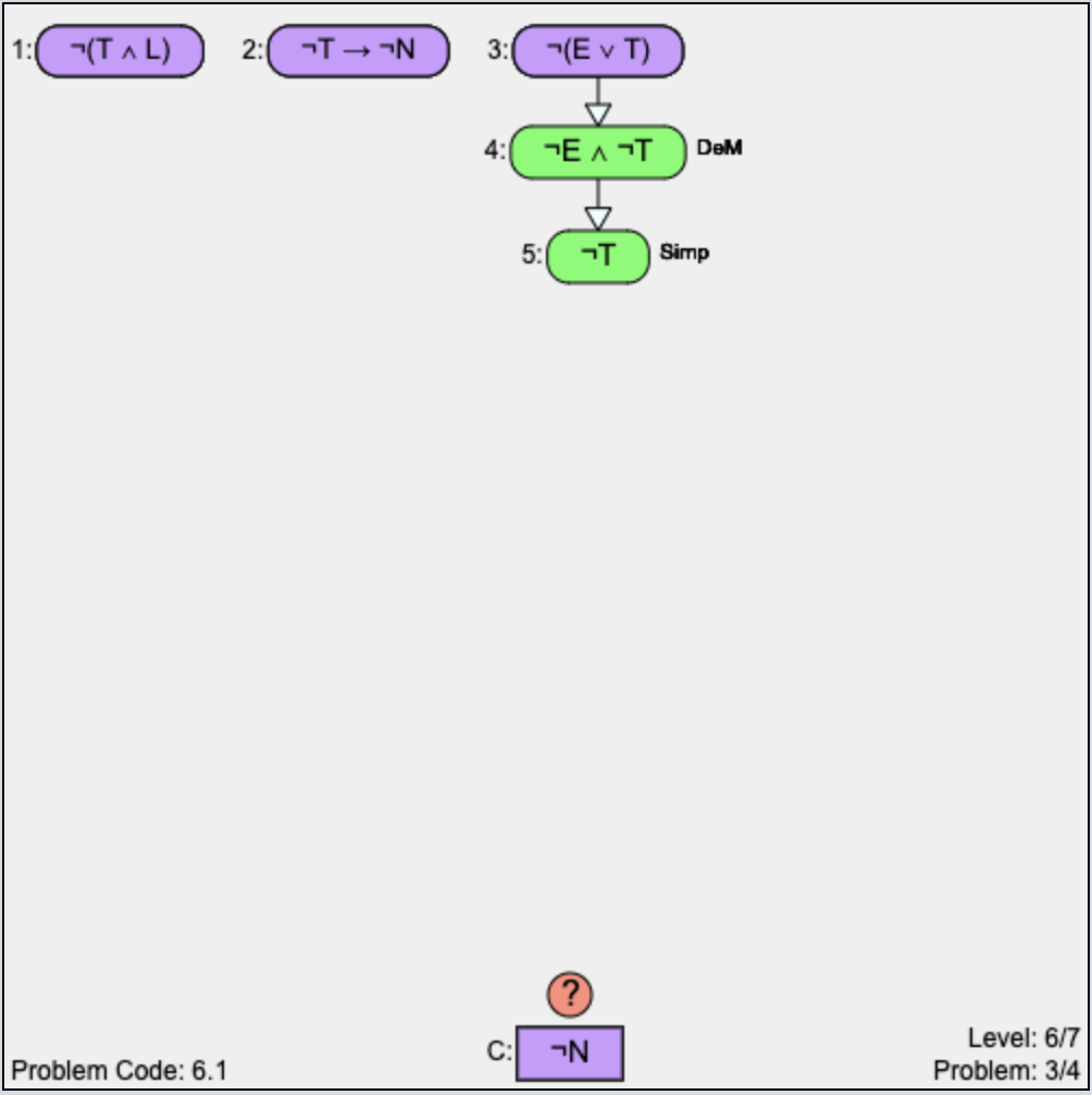
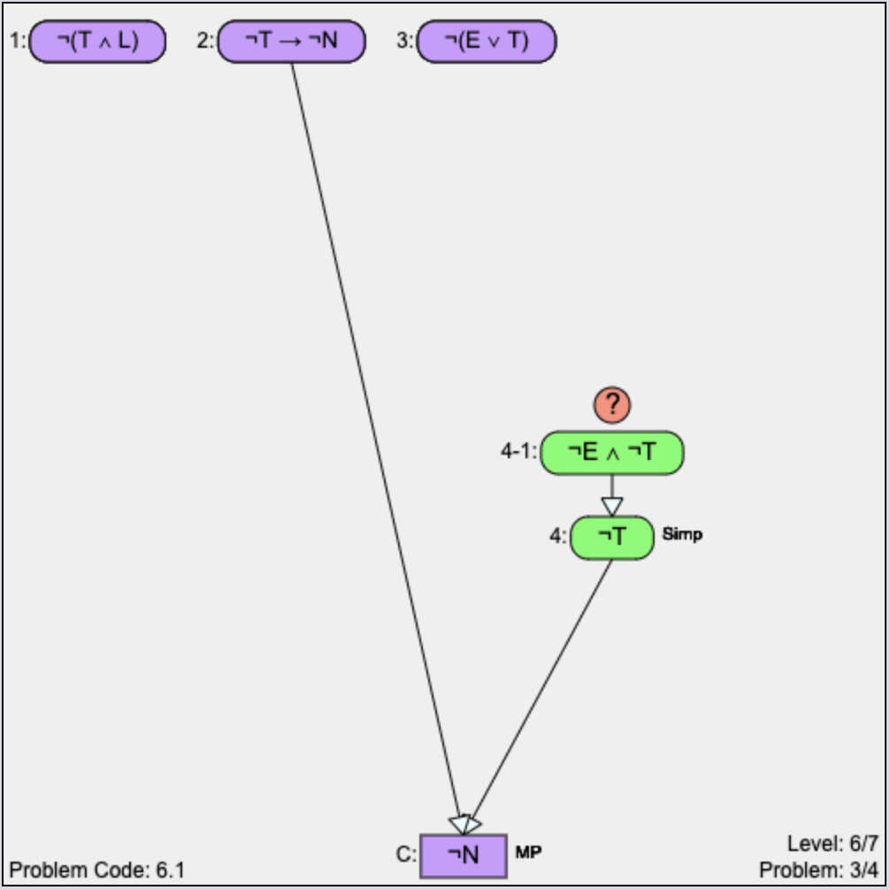
Backward Problem Solving: In this strategy (Figure 15b), proof construction progresses from the conclusion toward the given premises. At each step, the conclusion is refined to a new goal. In this strategy, students can add unjustified nodes in the proof that they wish to derive from the given premises. To derive a node backward, students need to select the ‘?’ button above a node, then select the rule, and then input the proposition(s) which are the antecedents of the selected node as per the selected rule. For example, in Figure 15b, the conclusion \(\neg N\) is first refined into antecedents \(\neg T\rightarrow \neg N\) and \(\neg T\) using the Modus Ponens (MP) rule. \(\neg T\rightarrow \neg N\) (given) is already justified. So, \(\neg T\) becomes the new goal since it is still unjustified. Then, \(\neg T\) is refined to a new goal \(\neg E\lor \neg T\) using the Simplification (Simp) rule. In this way, the unjustified goal(s) are refined to the given premises to complete the proof.
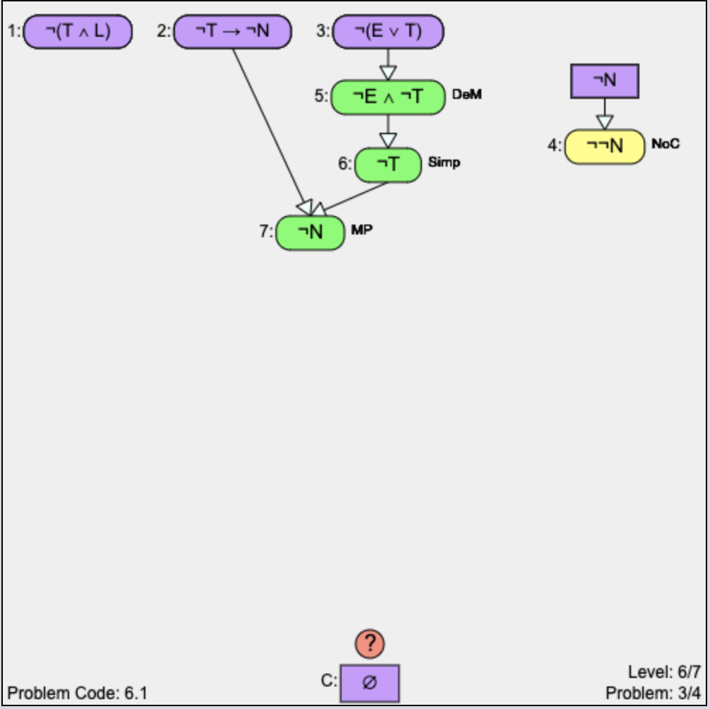
Indirect Problem Solving: Indirect problem solving [2] refers to the ‘Proof by contradiction’ approach. To construct a proof using this strategy, students first need to click on the ‘Change to Indirect Proof’ button (Figure 11) which adds the negation of the original conclusion to the list of givens (as in \(\neg \neg N\) in Figure 15c). From there, students need to derive two contradictory statements (for example, \(\neg \neg N\) and \(\neg N\)) to prove the contradiction (\(\emptyset \)).
Note that usually within Deep Thought, students are not required to follow any particular strategy. They can use any strategy at any point in a proof construction attempt.
B. SUPPLEMENTARY FIGURES
Figure 12, 13, and 14 supplement the analyses presented in Section 4.2.3 and 5.
1major propositions within a proof that can be used to decompose the proof, also referred to as Subgoals.
2The experts are two academic professionals with 10+ years of experience with logical reasoning
3In the pairwise tests each datapoint was used in at most three tests: (C, \(T_1\)), (C, \(T_2\)), and (\(T_1\), \(T_2\)). Thus, corrected \(\alpha \) = 0.05/3
4\(P_{MW}\)(\(T_2>T_1\)) refers to the p-value obtained from the Mann-Whitney U test for the hypothesis “\(T_2\) had significantly higher values than \(T_1\) for the metric under consideration." p \(<\) 0.016 indicates significance.
5The amount of working memory being used
6Unnecessary propositions are propositions that students derived during proof construction but later deleted and those were not part of the final proof.
© 2023 Copyright is held by the author(s). This work is distributed under the Creative Commons Attribution-NonCommercial-NoDerivatives 4.0 International (CC BY-NC-ND 4.0) license.