ABSTRACT
Randomized controlled trials (RCTs) in social or biomedical science often rely on covariate and outcome data drawn from a larger administrative database. For instance, a recent paired, clustered RCT of an online homework platform used covariates (demographics and prior achievement measures) and outcomes (standardized test scores) from the state’s educational database. To avoid confounding, typical analyses use only data from randomized subjects, discarding the remainder of the database.
In this study, we re-analyze data from the online homework study, substantially improving the precision of the effect estimates by using data from both randomized and non-randomized subjects. Our estimator does not introduce confounding and relies largely on standard modeling techniques. Specifically, we use observational data to train a random forest model predicting student test scores from student- and school-level covariates, and use it to generate predicted outcomes for students in the randomized schools. Then, we modify the hierarchical linear model from the original analysis by adding the predicted outcomes as an additional regressor, reducing the standard error by 15%—the improvement expected from increasing the sample size by over a third. Since it requires few additional modeling skills and no additional assumptions, this method can be easily adapted wherever auxiliary observational data are available.
Keywords
1. INTRODUCTION
In 2018, WestEd, an educational research agency, began a large-scale randomized field trial of the online mathematics application ASSISTments in 63 schools in North Carolina [3]. The researchers were granted access to the North Carolina student longitudinal data system, from which they drew most of the data used for the evaluation, including demographic and student achievement data from the students in the study—seventh-grade math students in the 63 randomized schools. However, the researchers had access to even more data: demographic, prior achievement, and outcome data from over 65 thousand additional 7th-grade students who attended North Carolina middle schools other than those 63.
The WestEd ASSISTments study is one example of a common phenomenon: covariate and outcome data for a randomized controlled trial (RCT) are drawn from a larger database that also includes data from similar subjects who were not randomized as part of the experiment. Other examples include A/B tests, which draw baseline covariates and outcomes from log data, and clinical trials, which draw baseline and outcome data from patients’ medical records. In these examples, researchers have access to big auxiliary observational datasets that are typically discarded or left unused. Granted, pooling data from randomized and non-randomized subjects would introduce confounding—there is no guarantee that subjects in the auxiliary data are comparable to the randomized subjects—and undermine the main motivation for conducting an RCT in the first place.
However, there are other uses for auxiliary observational datasets that maintain the integrity of the RCT. Specifically, [4] suggested using big auxiliary data to train a model predicting experimental outcomes, then using the resulting predictions as additional super-covariates in the “leave-one-out potential outcomes” (LOOP) effect estimator [23]. In studies of educational A/B tests, [4] and [19] showed that this approach can substantially reduce standard errors and increase statistical power, relative to estimators that do not use the auxiliary data. Similarly, [10] found similar results in a secondary analysis of a subset of school-aggregated data from a large, school-randomized effectiveness study, using a different, publicly available outcome than the original study.
These results are promising, but may not be fully convincing to education researchers conducting randomized field trials. First, we are unaware of any published analysis of a large randomized educational effectiveness study like [3] that uses auxiliary data as [4] proposes that uses the study’s primary outcome measure and includes data from the full RCT. Second, the method from [4] has been applied only to single-level data (or to multilevel data aggregated to the school level). In contrast, most large-scale educational efficacy studies use multilevel data, analyzing students as nested within schools. Third, previous studies have focused on the use of auxiliary data within the LOOP effect estimator, a new and unfamiliar estimator with limited availability and applicability, rather than incorporating insights from auxiliary data into familiar models.
In this paper, we present a secondary analysis of the WestEd ASSISTments study incorporating predictions from a random forest model trained on the auxiliary observational dataset composed of North Carolina students who did not participate in the original RCT. Our analysis uses the entire dataset from the original study, along with the study’s primary outcome measure, maintains and fully models the multilevel structure of the RCT dataset, and uses hierarchical linear modeling, the dominant approach for analyzing educational field trials, to estimate effects.
We find that, relative to the original estimates published in [3], our analysis reduces standard errors by 15%, roughly equivalent to increasing the number of schools in the study by 38%. Like previous auxiliary data methods, our approach does not introduce confounding and maintains the integrity of the randomization; unlike previous approaches, it is accessible to applied education researchers.
The following section describes the WestEd ASSISTments study of [3]. The next section reviews the relevant methodology, including the methods of [4] and hierarchical linear models. Section 4 describes our analysis, and Section 5 describes the results. Section 6 concludes.
2. THE ASSISTMENTS EFFICACY REPLICATION STUDY
ASSISTments [6] is an internet-based program for mathematics practice and learning, with a focus on middle school students. Teachers may draw from a large corpus of math problems—many drawn from popular curricula and textbooks—to create assignments for their classes. Students receive immediate feedback on the correctness of their work and often have access to hints or other tutoring materials. Teachers can monitor their students’ progress and browse useful data summaries for insights into student performance. A large, federally-funded randomized study conducted in Maine [14] showed that randomization to the ASSISTments condition increased student standardized test scores by \(0.22\pm 0.07\) standard deviations with 95% confidence.
Starting in 2018, WestEd conducted a replication study based in North Carolina, with the goal of extending the previous results to a more diverse population [3]. The study team matched 65 schools into 31 pairs and one triplet based on school-level demographics and prior achievement measures, and then randomly selected one school from each pair and two schools from the triplet for the treatment arm of the study. In those schools, all 7th-grade math teachers used ASSISTments for two academic years, 2018–2019 and 2019–2020, with teachers in the remaining 31 schools continuing business as usual. The original analysis plan was to use the 2019–2020 cohort’s end-of-grade mathematics state standardized test to measure efficacy. Unfortunately, due to the COVID-19 pandemic, the 2020 state standardized test was canceled. Fortunately, the study team was able to link the study data with student scores from a year after implementation ended, and estimate treatment effects using standardized test scores from the end of 8th grade. There were two different math standardized tests in 8th grade: the majority took the 8th-grade “end-of-grade” test (EOG08), while a subset of more advanced students took an Algebra I " end-of-course " exam. Following [3], our analysis focuses on the EOG08 exam, under the assumption that treatment assignment did not affect which exams students took. This assumption appears plausible: there was no evidence of differential attrition, and the analysis sample remained balanced on important covariates. All in all, the analysis sample includes 5,991 students, 3,030 randomized to the control condition, and 2,961 randomized to the treatment condition.
To estimate effects, the North Carolina Education Research Data Center granted the WestEd team access to demographic, achievement, and other educational data for all public school students in North Carolina. The study team selected covariates—including prior achievement measures at the student level (a math standardized test at the end of 6th grade, EOG6) and the school level (average 7th-grade scores from prior years), and demographics, including gender, race or ethnicity, and disability and economically disadvantaged status. They also calculated school-level demographics, including 7th-grade enrollment, whether the school was eligible for Title I funding, and the percentages of economically disadvantaged students and students from different ethnic groups. Following standard procedure, no use was made of covariate or achievement data from students in North Carolina schools that did not participate in the RCT.
The study’s main overall effect estimate was that randomization to ASSISTments in 7th grade caused an average impact of \(0.80\pm 0.64\) points on the EOG08 exam (with 95% confidence), corresponding to an effect size (Hedges’ \(g\)) of 0.10. Since the impact was measured a year after the intervention ended, this represents a persistent effect. See [3] for more details and estimated effects for subgroups.
3. METHODOLOGY BACKGROUND
Statistical analysis of RCTs requires data on the randomized condition, \(Z\)—which here we will take as binary, with \(Z_i=0\) if subject \(i\), \(i=1,\dots ,N^{RCT}\) is randomized to the control condition and \(Z_i=1\) if \(i\) is randomized to treatment—the outcome of interest, \(Y\), and, typically, a vector of covariates \(\bm {x}\). Covariates \(\bm {x}\), by definition, must be either fixed at baseline, i.e., at the time of randomization, or otherwise known to be independent of or invariant to randomization. Covariates are not always strictly necessary, but they can be invaluable for detecting, testing, and sometimes correcting irregularities in randomization, increasing the statistical precision of the effect estimate, and studying heterogeneity in causal impacts, and hence predicting treatment effects for future subjects or populations.
3.1 Observational Auxiliary Data
Data on \(Y\) and \(\bm {x}\) may be available for a separate sample of units that did not participate in the RCT. For instance, if researchers conducting an RCT drew data on \(\bm {x}\) and \(Y\) from a larger database that included, say, historical data or data on current units that were not randomized as part of the study. Along these lines, [20] discussed A/B tests run on ASSISTments E-trials [22], a platform for educational experiments within an online tool for middle-school mathematics practice. In that case, data on the outcome \(Y\), assignment completion, and covariates \(\bm {x}\) (students’ prior activities) were available for historical and concurrent users working on different parts of the platform. In this paper, we will re-analyze data from [3], a large educational field-trial testing the efficacy of ASSISTments in a set of North Carolina middle schools in which data on \(Y\), student scores on state standardized tests, and \(\bm {x}\), student demographics and prior standardized test scores, were drawn from the state department of education’s longitudinal data system. WestEd, which conducted and analyzed the RCT, was given access to the entire database and thus had access to data from students attending schools that were not part of the RCT.
Auxiliary observational data may seem of little use. In the cases just mentioned, data on the treatment condition \(Z\) are not available for students in the observational samples—we presume their experience was akin to the control condition, but this cannot be known. Even if data on the treatment or exposure were available in the observational sample, there would be good reasons not to use them — unlike in an RCT, exposure to the treatment or control conditions may be confounded. Furthermore, there is no guarantee that expected potential outcomes in the auxiliary data represent those in the RCT or even that the conditional distribution of outcomes given treatment status and covariates, \(p(Y|Z,\bm {x})\), is the same in the RCT and observational samples.
On the other hand, auxiliary observational data typically has a much larger sample size than an RCT, and could be helpful in modeling the conditional distribution of \(Y\) given \(\bm {x}\), enabling more precise effect estimation. Covariate data in [20] consisted of measurements from the sequence of assignments that students had worked on prior to the onset of the experiment—a complex longitudinal structure that was best modeled by a recurrent neural network that would be impossible or ill-advised to train from a small or moderately-sized RCT sample. The dataset in [3] is high-dimensional, longitudinal—including measurements from multiple successive years—and multilevel, since student data are nested within schools. A model fit only to RCT data would be unable to capture those complexities fully. Moreover, even if RCT data were large enough to support modern ML models, incorporating such a model into a causal effect estimator poses its own challenges, especially when the ML model cannot be guaranteed to be unbiased, as is typically the case.
Recent literature [12, 17, 4, 20] suggests an approach to using big observational data to model the relationship between \(\bm {x}\) and \(Y\) and then incorporating that relationship into an RCT analysis without requiring additional untestable assumptions regarding the auxiliary data or the ML model and without introducing any confounding bias. The idea is, essentially, to use the observational data to train a supervised learner predicting \(Y\) as a function of \(\bm {x}\); to use that pretrained model, along with \(\bm {x}\) data from RCT subjects, to generate predicted outcomes \(\hat {y}^{obs}\) for RCT subjects; and finally to statistically adjust for \(\hat {y}^{obs}\) in an effect estimator. The predictions \(\hat {y}^{obs}\) act as a one-dimensional summary of multidimensional covariates \(\bm {x}\), where the summary was designed to extract as much relevant information about \(Y\) as possible. Because it is based on RCT covariates \(\bm {x}\) and a model trained on an external dataset, \(\hat {y}^{obs}\) are independent of \(Z\)—in other words, \(\hat {y}^{obs}\) itself is a covariate.
Ideally, \(\hat {y}^{obs}\) will be closely correlated with observed outcomes \(Y\) within each treatment group—in other words, the auxiliary-data model closely predicts RCT outcomes. A subject’s treatment effect, by definition, is the difference between that subject’s observed outcome \(Y_i\) and the counterfactual outcome, or what would have been observed if \(i\) had been randomized to the other treatment. Hence, accurate predictions of counterfactual outcomes can increase statistical precision and power when estimating average treatment effects. However, when \(\hat {y}^{obs}\) are only weakly correlated with \(Y\), or even anti-correlated, methods described in [4, 20] ensure that the effect estimates remain exactly unbiased and (approximately in small samples, exactly in large samples) no less precise than unbiased estimators that do not use auxiliary data.
Unfortunately, the specific methods recommended in those papers
may not always be applicable or practical. [4, 20] recommend
adjusting treatment effect estimation with a powerful but
somewhat complex method [23, 24] that is currently only
available for Bernoulli or paired individually-randomized trials
and for paired group randomized trials in which covariates and
outcomes are aggregated to the group level [9]. Moreover, these
may be unfamiliar or inaccessible to most applied researchers
(they are currently implemented only in an experimental R
package [8]).
3.2 Group-Randomized Trials and Hierarchical Linear Models
Multilevel structures are a hallmark of K–12 education: students are nested within classrooms, which are nested within schools. It is often impractical or impossible to randomize classmates or schoolmates into different educational conditions, so a common technique in experimental education research is to randomize entire classrooms or schools between conditions [11, 15, 3]. In these cases, every student in a single classroom or school is randomized to the same condition, either treatment or control. Educational outcomes tend to be correlated among students within the same school [5], so it is crucial to account for the clustered-randomization design when analyzing clustered RCTs, for instance, by using school-average outcomes to estimate effects [9].
However, researchers often prefer to maintain their data’s multilevel structure by using models that explicitly account for within-school correlations. In educational effectiveness research, the most common of these is the hierarchical linear model (HLM) [13]—or, more precisely, a random intercept model—such as:
where the subscript \(s[i]\) indicates student \(i\)’s school, \(\alpha _0\) is an overall intercept, \(\bm {w}_s\) are school-level covariates, and \(\eta _s\sim N(0,\sigma ^2_{scl})\) and \(\epsilon \sim N(0,\sigma _{ind}^2)\) are school- and student-level regression errors, with variances \(\sigma _{scl}^2\) and \(\sigma _{ind}^2\) estimated from the data. When schools are paired prior to randomization—so that one school from each pair is randomized to treatment, and the other to control, as in [3]—pair indicators are included in \(\bm {w}\).
The coefficient \(\tau \) represents the estimated treatment effect—the extent to which student scores in treated schools vary, on average, from scores in control schools, conditional on covariates and other school-level factors.
In an HLM such as \eqref{eq:hlm}, student scores \(Y_i\) are modeled as varying based on their school, via \(\eta _s\), \(\bm {w}_s\) and \(Z_s\), and individual characteristics \(\bm {x}\). Since treatment is assigned at the school level, the treatment indicator \(Z\) has a subscript \(s\) and appears in the school-level model of \eqref{eq:hlm}. Student scores \(Y\) are assumed to be independent conditional on regressors \(\bm {x}\), \(Z\), and \(\bm {w}\) and school errors \(\bm {\eta }\); the school intercepts, in turn, are independent of each other conditional on \(Z\) and \(\bm {w}\). Finally, conditional on \(\bm {x}\), \(Z\), and \(\bm {w}\), student scores \(Y_i\) and \(Y_j\) are independent for students in different schools, \(s[i]\ne s[j]\) but correlated with “intraclass correlation coefficient” \(\rho =\sigma _{sch}^2/(\sigma _{sch}^2+\sigma _{ind}^2)\) for two students in the same school. Hence, HLMs explicitly account for student correlation within schools and are therefore appropriate for school-randomized studies.
4. METHOD
The student-level data used in this study were confidential; hence, all analyses were conducted at WestEd, using Stata.
We followed a two-step procedure to estimate average effects:
- 1.
- Use the observational data to train a random forest [2] using baseline covariates to predict student test scores, and use that fitted model to predict test scores for students in the RCT.
- 2.
- Estimate average treatment effects by fitting a hierarchical linear model to RCT data, including the predictions from step 1 as a regressor.
The following sections will describe each of these steps in detail.
4.1 Predicting Student Test Scores
As described in Section 2, the research team had access to student-level data from across North Carolina. We used this database to compile an observational auxiliary dataset for training a model to predict students’ EOG08 test scores.
First, we identified 65,658 North Carolina middle school students who were not part of the RCT and took the 2021 EOG08 exam. We used anonymized records from all of these students to compile an observational auxiliary dataset. Specifically, we first assembled relevant baseline covariates; since the experiment took place when students were in 7th grade, we restricted covariates to measurements recorded when students were in 6th grade or earlier. These included 6th-grade student background data—age; status as academically gifted, disabled, economically disadvantaged, and/or English language learner; ethnicity indicators; and whether a student was in foster care, homeless, a migrant, and/or connected to the military. We also included students’ reading and math assessments from grades 3-6, and 5th-grade science assessments.
We suspected that school characteristics may predict student outcomes, even beyond individual student predictors. Hence, we calculated additional school-level features to include in the random forest. Specifically, we calculated the percentage of students at each school and grade level (grades 3–6) who belonged to each demographic category, as well as the school-grade-level average math, reading, and science assessment scores. All in all, this amounted to 94 student- and school-level features per student.
After compiling the covariates, we fit a random forest regression
model to predict students’ EOG08 scores. We fit the model
using the rforest command in Stata [21], using the system
default tuning parameters (i.e., investigate 9 variables per split
and 100 iterations). The random forest predicted posttest scores
in the auxiliary data with high accuracy: the out-of-bag
prediction \(R^2\) was roughly 0.92.
Finally, we used the fitted model to predict EOG08 math test scores for students in the RCT sample.
As argued above, these predictions, \(\hat {y}^{obs}\), can be considered baseline covariates: they were constructed using RCT students’ measurements from 6th grade or earlier, and a model fitted to an external sample. Hence, they were invariant to the randomized treatment assignment in the RCT.
4.2 Estimating Treatment Effects
To estimate average treatment effects, we simply re-ran the HLM from the original analysis with \(\hat {y}^{obs}\) as an additional covariate, and reported the coefficient on the treatment randomization indicator, along with its standard error.
That is, we compared the original HLM of [3] with an HLM that included \(\hat {y}^{obs}\) as an additional student-level predictor (i.e., an additional column of \(\bm {x}\) in 1), and was otherwise identical.
In exploratory analyses, we compared our main estimator with an alternative in which \(\hat {y}^{obs}\) replaces prior test scores EOG06, rather than supplementing it. That is, we fit an additional HLM that includes \(\hat {y}^{obs}\) as a predictor but excludes EOG06. Since both \(\hat {y}^{obs}\) and EOG06 are predictors of EOG08, including both in the model may lead to collinearity and inflate standard errors.
5. RESULTS
5.1 Predicting 8th Grade Scores from Observational Data
The random forest accurately predicted EOG08 scores: the out-of-bag root mean squared error was 2.1 points, corresponding to a pseudo-\(R^2\) of roughly 93%. By comparison, an analogous linear regression model had a root-mean-square error of 2.6.
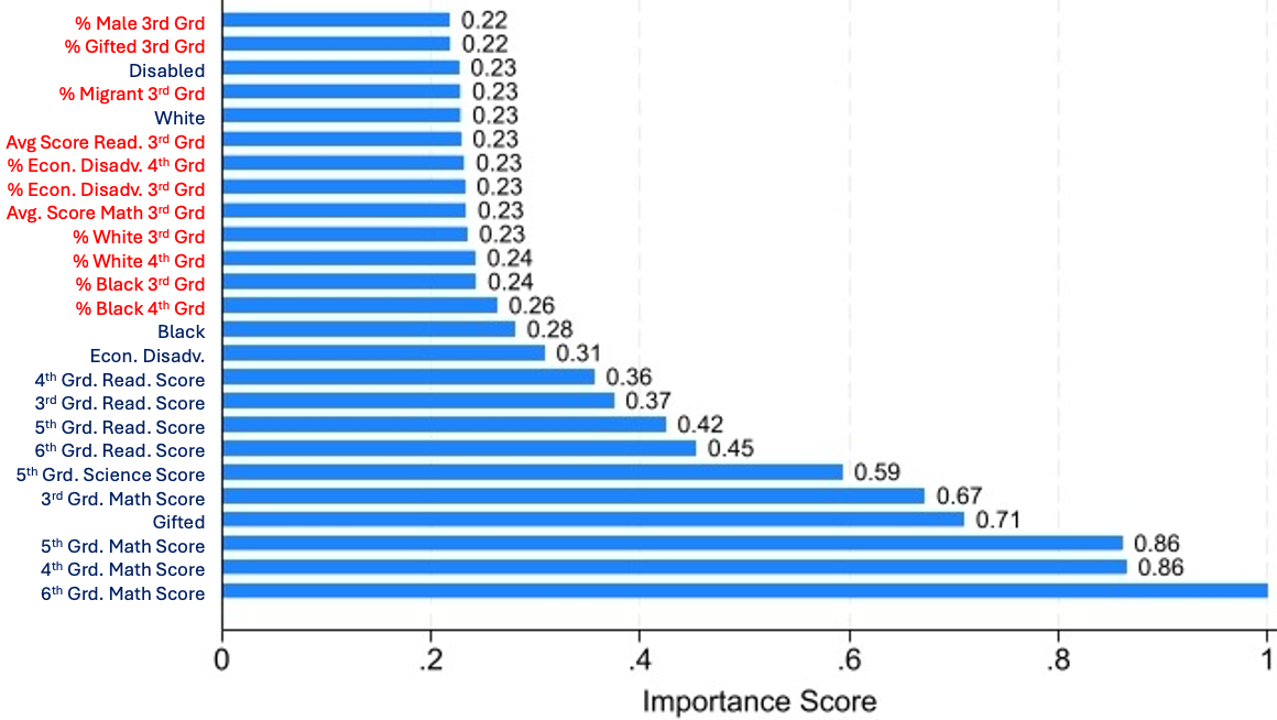
Figure 1 shows a variable importance measure for the top 25 most important predictors in the random forest. In this case, a predictor’s importance is the average decrease in mean squared error across splits based on that predictor in the component trees of the random forest. The values in Figure 1 are divided by the importance measure for the most important predictor, 6th grade math score, so that they range from 0–1 [21].
The three most important predictors, by this measure, are the students’ three prior math standardized test scores, followed by previous reading scores and other student-level variables. Most of the remaining top 25 variables are school-level aggregates, including school demographics and prior average exam scores. Notably, only two of the top ten and six of the top 25 predictors appeared in the original HLM (the 6th-grade math score and individual demographics), suggesting that the random forest identified important predictors previously underappreciated. Specifically, students’ prior math scores from 4th and 5th grade and their prior reading scores seem to play an important role.
5.2 Estimating Effects
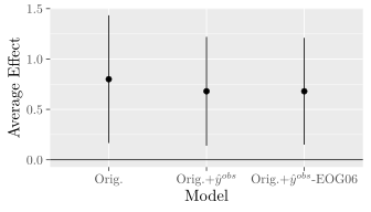
Table 1 and Figure 2 show estimated effects from the original model from [3] alongside two modified models: with \(\hat {y}^{obs}\) as an additional predictor and with \(\hat {y}^{obs}\) replacing students’ prior scores, EOG06.
Including \(\hat {y}^{obs}\) as an additional predictor decreased the standard error by 15%, from 0.317 to 0.270. Since standard error tends to be inversely proportional to the square root of the sample size, decreasing the standard error by this amount is roughly equivalent to increasing the sample size by 38%, a substantial improvement.
If \(\hat {y}^{obs}\) replaces EOG06 in the HLM (i.e., if EOG06 is dropped from the model), the standard error decreases even more, to 0.265, a decrease of over 16%, corresponding to a 44% increase in effective sample size.
| Model | Eff. | SE | Hedges’ g | p |
| Orig. | 0.80 | 0.317 | 0.10 | 0.012 |
| Orig.\(+\hat {y}^{obs}\) | 0.68 | 0.270 | 0.08 | 0.011 |
| Orig.\(+\hat {y}^{obs}\)-EOG06 | 0.68 | 0.265 | 0.08 | 0.011 |
6. DISCUSSION
In re-analyzing data from a recent large educational efficacy study, this paper described a method for incorporating data from across the state, including students from both randomized and non-randomized schools. The method combines insights from recent statistical literature [4] with more conventional hierarchical linear modeling, and captures many of the advantages of both: it uses observational data to increase statistical power and precision without introducing confounding bias, it uses familiar and flexible methods that are accessible to applied education researchers, and it fully models the hierarchical structure of the data. In the analysis presented here, incorporating observational data was equivalent to increasing the sample size by over a third.
The results presented here represent the beginning of our reanalysis of the North Carolina data. Future research will apply the method described here to estimate the effect of randomization on the more advanced "end of course" exam, as well as on students’ choice to take one exam or the other—did assignment to the treatment condition cause some students to take the more (or less) advanced 8th grade class? We also hope to delve deeper into the random forest model discussed in Section 5.1 to better understand its superiority to more parsimonious linear models. Finally, we hope to use the method discussed here to estimate subgroup effects; hopefully, the additional power will enable the investigation of smaller subgroups.
In general, we hope that future research will apply this method to other datasets to better understand how often and by how much incorporating auxiliary data can improve statistical power. Ideally, the availability of auxiliary data can help researchers conduct smaller experiments—first, they will need a tool to prospectively estimate the power gains from auxiliary data, perhaps akin to [7].
Overall, the larger the (absolute) correlation between \(\hat {y}^{obs}\) and the outcomes \(Y\) in the RCT sample, the greater the resulting gains in precision will be. In the worst case, when the correlation is low or zero, incorporating \(\hat {y}^{obs}\) into a causal estimator may increase standard errors slightly—like adding any noise covariate to the model—and will not cause bias.
These considerations imply that choosing a better-performing predictive model can lead to more precision gains. In this study, we used the random forest, which has shown competitive performance in previous research [10], and is relatively easy to implement, but a better model would have led to even greater precision gains. Fortunately, auxiliary data can be used to both train and select the predictive model: since it is a completely separate dataset from the RCT, it can serve as a sandbox for attempting various predictive models and choosing between them. However, the model’s performance in the RCT sample, where it counts, may be substantially lower than in the auxiliary data; we are actively researching and developing transfer learning models that may mitigate this issue.
Since precision gains are driven by the correlation between \(\hat {y}^{obs}\) and \(Y\), and not predictive accuracy, our approach, properly tweaked, may work even if the outcome in the auxiliary data is not the same as in the RCT, but is correlated. Our first attempts in this direction were not encouraging [18], but the work is ongoing.
The method described here is an example of data fusion, a growing interest among quantitative researchers in integrating observational and randomized data [1, 16]. These include methods for extrapolating RCT results to other populations, identifying important moderators or mediators, as well as methods, like the one discussed here, for increasing precision and power. Data fusion is an exciting new direction in statistical causal inference, and it is especially relevant to educational data mining. We hope that as more methods and datasets become available, incorporating randomized and non-randomized data into unified analyses will accelerate the science of learning.
7. ACKNOWLEDGMENTS
The research reported here was supported by the Institute of Education Sciences, U.S. Department of Education, through Grant R305D210031. The opinions expressed are those of the authors and do not represent views of the Institute or the U.S. Department of Education.
The authors are grateful for helpful comments from Charlotte Z. Mann, Jaylin Lowe, Yanping Pei, three anonymous reviewers, and a metareviewer. The authors are also grateful to Neil Heffernan for all sorts of things, including, but not limited to, ideas, encouragement, and string-pulling—and, by extension, Angela Kao, without whom none of this would have gotten done.
8. REFERENCES
- E. Bareinboim and J. Pearl. Causal inference and the data-fusion problem. Proceedings of the National Academy of Sciences, 113(27):7345–7352, 2016.
- L. Breiman. Random forests. Machine learning, 45:5–32, 2001.
- M. Feng, N. Brezack, C. Huang, and K. Collins. Long-term effects of an online math tool on us adolescents’ achievement. British Journal of Educational Technology, 2025.
- J. A. Gagnon-Bartsch, A. C. Sales, E. Wu, A. F. Botelho, J. A. Erickson, L. W. Miratrix, and N. T. Heffernan. Precise unbiased estimation in randomized experiments using auxiliary observational data. Journal of Causal Inference, 11(1):20220011, Jan. 2023. Publisher: De Gruyter.
- L. V. Hedges and E. C. Hedberg. Intraclass correlation values for planning group-randomized trials in education. Educational Evaluation and Policy Analysis, 29(1):60–87, 2007.
- N. T. Heffernan and C. L. Heffernan. The assistments ecosystem: Building a platform that brings scientists and teachers together for minimally invasive research on human learning and teaching. International Journal of Artificial Intelligence in Education, 24(4):470–497, 2014.
- J. Lowe, C. Z. Mann, J. Wang, A. Sales, and J. A. Gagnon-Bartsch. Power calculations for randomized controlled trials with auxiliary observational data. In B. Paaßen and C. D. Epp, editors, Proceedings of the 17th International Conference on Educational Data Mining, pages 469–475, Atlanta, Georgia, USA, July 2024. International Educational Data Mining Society.
- C. Mann, E. Wu, A. Sales, and J. Gagnon-Bartsch. dRCT: Design-Based Covariate Adjustment for the Average Treatment Effect, 2025. R package version 1.0.0, commit d423d3de8f3befe78328d6bbd124916ecf7c7195.
- C. Z. Mann, A. C. Sales, and J. A. Gagnon-Bartsch. A general framework for design-based treatment effect estimation in paired cluster-randomized experiments. arXiv preprint arXiv:2407.01765, 2024.
- C. Z. Mann, J. Wang, A. Sales, and J. A. Gagnon-Bartsch. Using publicly available auxiliary data to improve precision of treatment effect estimation in a randomized efficacy trial. In B. Paaßen and C. D. Epp, editors, Proceedings of the 17th International Conference on Educational Data Mining, pages 518–525, Atlanta, Georgia, USA, July 2024. International Educational Data Mining Society.
- J. F. Pane, B. A. Griffin, D. F. McCaffrey, and R. Karam. Effectiveness of Cognitive Tutor Algebra I at Scale. Educational Evaluation and Policy Analysis, 36(2):127–144, 2014. Publisher: [American Educational Research Association, Sage Publications, Inc.].
- T. Patikorn, D. Selent, N. T. Heffernan, J. E. Beck, and J. Zou. Using a single model trained across multiple experiments to improve the detection of treatment effects. International Educational Data Mining Society, 2017.
- S. Raudenbush and A. Bryk. Hierarchical linear models: Applications and data analysis methods. Sage, Chicago, 2002.
- J. Roschelle, M. Feng, R. F. Murphy, and C. A. Mason. Online mathematics homework increases student achievement. AERA Open, 2(4):2332858416673968, 2016.
- J. Roschelle, M. Feng, R. F. Murphy, and C. A. Mason. Online mathematics homework increases student achievement. AERA open, 2(4):2332858416673968, 2016.
- E. T. Rosenman. Methods for combining observational and experimental causal estimates: A review. Wiley Interdisciplinary Reviews: Computational Statistics, 17(2):e70027, 2025.
- A. C. Sales, A. Botelho, T. M. Patikorn, and N. T. Heffernan. Using big data to sharpen design-based inference in a/b tests. In K. E. Boyer and M. Yudelson, editors, Proceedings of the 11th International Conference on Educational Data Mining. (EDM 2018), pages 479–486. International Educational Data Mining Society, 2018.
- A. C. Sales, C. Mann, J. Gagnon-Bartsch, and N. Heffernan. Effect estimates using publicly available school- level data in a cluster-randomized educational experiment. In Proceedings of the 18th International Conference on Educational Data Mining, pages 578–581. International Educational Data Mining Society, July 2025.
- A. C. Sales, E. B. Prihar, J. A. Gagnon-Bartsch, and N. T. Heffernan. Using auxiliary data to boost precision in the analysis of a/b tests on an online educational platform: New data and new results. Journal of Educational Data Mining, 15(2):53–85, 2023.
- A. C. Sales, E. B. Prihar, J. A. Gagnon-Bartsch, N. T. Heffernan, et al. Using auxiliary data to boost precision in the analysis of a/b tests on an online educational platform: New data and new results. Journal of Educational Data Mining, 15(2):53–85, 2023.
- M. Schonlau and R. Y. Zou. The random forest algorithm for statistical learning. The Stata Journal, 20(1):3–29, 2020.
- A. Siedahmed, Y. Pei, A. C. Sales, N. T. Heffernan, J. Gagnon-Bartsch, D. Zhang, B. A. Schuetze, and A. Zengilowski. E-trials: Empowering data-driven decisions to enhance computer-based learning platforms. arXiv preprint arXiv:2502.10545, 2025.
- E. Wu and J. A. Gagnon-Bartsch. The loop estimator: Adjusting for covariates in randomized experiments. Evaluation review, 42(4):458–488, 2018.
- E. Wu and J. A. Gagnon-Bartsch. Design-based covariate adjustments in paired experiments. Journal of Educational and Behavioral Statistics, 46(1):109–132, 2021.
© 2026 Copyright is held by the author(s). This work is distributed under the Creative Commons Attribution-NonCommercial-NoDerivatives 4.0 International (CC BY-NC-ND 4.0) license.