ABSTRACT
Knowledge Tracing (KT) models are essential for estimating student knowledge states, yet prominent attention-based architectures like SAINT and SAKT struggle with length extrapolation, often failing when sequence lengths exceed those seen during training. This limitation frequently arises from the use of absolute learnable positional embeddings. Furthermore, existing methods often treat interactions as uniformly spaced, failing to capture the continuous temporal dynamics of learning and forgetting. This paper investigates the incorporation of Time-and-Order rotation Positional Encoding (TO-RoPE), which treats both discrete interaction order and continuous real time as geometric properties of the latent space. By applying deterministic rotations to queries and keys, TO-RoPE allows for robust extrapolation to longer sequences while capturing heterogeneous temporal patterns. We conducted an empirical study across three datasets: ASSISTments2017, EdNet, and a Proprietary Dataset. The results demonstrate that replacing absolute embeddings with TO-RoPE significantly improves the AUC performance of SAINT and SAKT in extrapolated windows of up to 500 interactions. In particular, the SAINT + TOR configuration consistently outperformed the baselines, suggesting that explicit geometric modeling of continuous time is a viable approach to modeling long-range dependencies in digital education environments.
Keywords
1. INTRODUCTION
The aim of personalized education at scale is fundamentally based on our ability to model learners’ evolving cognitive states [30]. Knowledge Tracing (KT), the computational task of predicting student future performance based on historical interactions, serves as the analytical engine for personalized solutions, such as Intelligent Tutoring Systems (ITS) and Adaptive Systems [2, 16]. By accurately mapping a student’s mastery over specific Knowledge Components (KCs), these systems can transition from static, one-size-fits-all curricula to adaptive environments that provide targeted feedback and optimized learning paths. Furthermore, educational platforms have begun to generate large volumes of data on student interactions, opening opportunities for analytical techniques to enhance the learning experience [23, 11, 3].
In this context, recent breakthroughs in Deep Learning, particularly with Transformer-based architectures such as SAINT and SAKT, have established new benchmarks in KT by using self-attention to capture complex dependencies across student histories [8, 9, 19]. However, these models share a structural dependency on absolute positional embeddings, which treat student interactions as a rigid, equidistant sequence. This approach fundamentally ignores the temporal reality of human learning, in which the time between interactions carries essential information about memory consolidation, interference from external activities, and the inevitable decay of knowledge [28]. Although previous efforts like AKT and LefoKT introduced temporal biases or handcrafted decay functions to mitigate this, they largely treat time as a discrete proxy rather than a continuous intrinsic property of the learning process [14, 5].
On the other hand, the reliance on absolute positions further restricts the models’ capacity for length extrapolation. In typical research settings, KT models are trained and validated in truncated interaction windows [2]. However, a truly effective KT system is expected to maintain predictive stability throughout a student’s entire academic tenure [13]. As a result, rather than the technical challenge of processing longer sequences, length extrapolation is required for reliable long-term performance predictions [17]. That is, if the predictive accuracy of a model degrades simply because a student has exceeded the interaction count seen during the training phase, the system becomes an unreliable guide for high-stakes longitudinal outcomes, such as identifying early risks of course failure or certifying long-term retention [30].
To bridge this gap, this study investigates a new approach to positional and temporal encoding by integrating Time-and-Order rotation Positional Encoding (TO-RoPE) [27]. By encoding positions as relative rotations in a complex-valued latent space, TO-RoPE provides a theoretically grounded mechanism for both length extrapolation and continuous-time modeling. Unlike additive embeddings, which anchor the model to a fixed coordinate system, rotation encodings allow the attention mechanism to perceive the distance between interactions, both in terms of sequential order and in terms of actual time elapsed, as a relative geometric property. This potentially enables models trained on short interaction windows to generalize seamlessly to the much longer sequences characteristic of real-world educational data.
Therefore, this work evaluates whether substituting absolute embeddings with a dimension-separated TO-RoPE strategy can enhance the robustness of attention-based KT models. To this end, we developed new versions of the SAINT and SAKT architectures to isolate the effects of this geometric encoding and subject them to a rigorous train-short, test-long protocol. Thus, our main contribution lies in demonstrating how this approach affects the extrapolation of student mastery over extended periods and across varying temporal scales. By validating our findings across three diverse datasets, ranging from controlled mathematics tutoring (ASSISTments2017 [4]) to large-scale TOEIC preparation (EdNet [10]) and a proprietary higher-education dataset, we provide evidence for a more scalable and temporally aware framework for KT.
2. BACKGROUND
The KT problem is formally defined as a sequence-processing task aimed at modeling dependencies between past interactions of a student to predict future performance [30, 16]. Given an interaction history:
where \(q_i\) represents the question, \(a_i \in \{0,1\}\) the correctness, and \(\tau _i\) the timestamp, KT models estimate the probability of correctness for a future question \(q_t\):
These estimates are fundamental for adaptive educational systems [2].
2.1 Attention-based Knowledge Tracing
The introduction of the self-attention mechanism [25] revolutionized KT by enabling modeling of long-range dependencies without the vanishing gradient limitations of recurrent neural networks (RNNs), such as deep knowledge tracking (DKT) [21].
Pandey et al. [19] pioneered this approach with Self-Attentive Knowledge Tracing (SAKT), an encoder-only architecture in which the current exercise serves as a query to retrieve relevant past interactions. Subsequently, Choi et al. [9] proposed SAINT, a Transformer-based encoder-decoder model that processes exercises and responses separately.
However, both SAKT and SAINT rely on learnable absolute positional embeddings to encode interaction order. In SAINT, for instance, position is handled by adding a learned vector \(\mathbf {P}_i\) to the input:
A critical limitation of this approach is the lack of length extrapolation. Since \(\mathbf {P}_i\) is learned for specific indices \(i \in [0, L_{train}]\), these models fail to generalize when a student’s history exceeds the duration of the training window \(L_{train}\), which is a frequent scenario on lifelong learning platforms. Consequently, when \(t > L_{train}\), the model lacks a defined positional representation, leading to performance degradation.
2.2 Time-aware Knowledge Tracing
To address the irregularity of learning sessions, several works have incorporated temporal information into attention mechanisms. Ghosh et al. [14] proposed Attentive Knowledge Tracing (AKT), which introduces a monotonic attention mechanism with exponential decay. This method modulates attention weights based on the temporal distance between interactions, reflecting the cognitive effect of forgetting.
More recently, Bai et al. [5] introduced LefoKT, which employs a relative forgetting attention mechanism. LefoKT adds a bias term \(B_{i,j}\) to the attention logits, penalizing older interactions:
Although AKT and LefoKT successfully incorporate temporal biases, they treat time primarily as a scalar penalty (a decay factor or additive bias) applied to the attention scores. This approach imposes an explicit monotonic decay, restricting their capacity to capture complex temporal dynamics, such as non-monotonic forgetting patterns and study periodicity. Furthermore, these models often still anchor their notion of time in discrete ordinal indices.
2.3 Geometric Positional Encodings
To overcome the limitations of absolute embeddings and scalar biases, recent advances in Large Language Models (LLMs) have explored encoding position directly into the geometry of the latent space. Rotating positional embedding (RoPE) [22] proposes that the inner product between a query and a key should depend only on their relative distance. Instead of adding a positional vector, RoPE rotates the affine-transformed word embeddings by an angle proportional to their position.
This rotation ensures that the attention score \(Q K^\top \) naturally captures relative distances, allowing the model to generalize to sequence lengths significantly larger than those seen during training (length extrapolation).
Wei et al. [27] extended this concept to irregular time series with Time-and-Order RoPE (TO-RoPE). Recognizing that discrete order is insufficient for processes with irregular intervals, TO-RoPE treats both discrete order (\(i\)) and continuous time (\(\tau \)) as sources of rotation. By interpolating these two dimensions, the model encodes the distance between interactions as a composite geometric property in a complex vector space.
To the best of our knowledge, the integration of Time-and-Order RoPE into the Knowledge Tracing domain remains unexplored. Although existing models like AKT and LefoKT address temporal dynamics through decay mechanisms, they do not leverage the geometric properties of the latent space to model continuous time. This work bridges this gap by replacing absolute positional embeddings in SAKT and SAINT with TO-RoPE, hypothesizing that treating both order and time as rotational components will unlock superior length extrapolation capabilities and more robust temporal modeling.
2.4 Research Questions
As detailed in Section 2, current Knowledge Tracing architectures face a fundamental structural dichotomy: they either rely on absolute positional embeddings that bind the model to fixed sequence lengths (as in SAINT and SAKT) or attempt to patch temporal dynamics through decay mechanisms or additive scalar biases (as in AKT and LefoKT). However, these methods treat time predominantly as an auxiliary bias rather than an intrinsic, continuous dimension of the latent space. In this work, we propose shifting the modeling paradigm from additive embeddings to Time-and-Order rotation Positional Encoding (TO-ROPE), postulating that encoding both sequence order and continuous elapsed time as geometric rotations offers a superior inductive bias. To validate this hypothesis, we investigate two critical dimensions of model performance: the capacity for length generalization and the interpretability of learned temporal patterns.
A primary failure of absolute positional embeddings, as described in Section 2.1, is the use of fixed training windows. Because position vectors are learned for specific indices (\(i \in [0, L_{train}]\)), standard models lack a defined representation of student histories that exceed the window size observed during training—a scenario inherent to lifelong learning platforms. We investigate whether replacing this fixed coordinate system with relative rotation encodings allows the model to decouple predictive capability from absolute positions, thereby maintaining stability over indefinitely long sequences. As such, the first research question is:
Research Question 1 (RQ1):
To what extent does replacing absolute positional
embeddings with Time-and-Order RoPE enable
attention-based Knowledge Tracing models to
extrapolate predictive performance to sequence
lengths significantly exceeding those observed
during training?
Furthermore, although previous work explicitly enforces temporal forgetting via monotonic decay biases (Section 2.2), it remains unclear whether a model can naturally learn these dynamics solely from geometric constraints. By treating continuous time as a rotational dimension in the complex plane, the attention mechanism can dynamically discern the temporal distance between interactions. We aim to determine whether this geometric encoding leads to the spontaneous emergence of coherent attention distributions that reflect realistic cognitive phenomena—such as knowledge decay—without relying on handcrafted penalty functions.
Research Question 2 (RQ2):
How does the incorporation of continuous time
as a geometric property of the latent space
influence the model’s attention mechanisms, and
does it yield interpretable temporal decay patterns
distinct from those derived solely from discrete
ordinal indices?
3. METHOD

To address the proposed research questions and isolate the effects of positional encoding from other architectural variables, we utilize the established state-of-the-art models SAINT and SAKT as our baseline frameworks. These models were specifically selected for their benchmark performance in the literature [2] and their reliance on absolute positional embeddings. Unlike models such as AKT or LefoKT [14, 5], SAINT and SAKT do not incorporate explicit temporal decay mechanisms. By replacing their original positional mechanisms with TO-RoPE, we can directly observe the impact of geometric temporal encoding without interference from auxiliary decay components. The following section describes the model architecture.
3.1 Positional Encoding Adjustment
Standard Transformer-based KT models are based on additive absolute positional embeddings [2]. We modify the input formulation to remove these explicit position vectors (\(P_i\)), forcing the model to rely solely on the rotation mechanism for sequence information.
SAINT ReformulationIn the original SAINT architecture, the position is added as an absolute learnable vector in the response and exercise embeddings. We simplify the input representation for the encoder (\(\mathbf {E}\)) and the decoder (\(\mathbf {R}\)) as follows:
Where \(\mathbf {kc}_i\), \(\mathbf {q}_i\), \(\mathbf {a}_i \in R^d\), represent, respectively, the embedding for the Knowledge Component, Question ID, and answer correctness at step \(i\) and \(d\) the dimension of the latent space. Note that the positional term \(\mathbf {P}_i\) is explicitly removed.
SAKT ReformulationSimilarly for SAKT, we remove the positional embedding from the interaction matrix formulation. The activity matrix (\(\mathbf {E}\)) remains unchanged, while the interaction matrix (\(\hat {\mathbf {M}}\)) is defined as:
Where \(\mathbf {M}_{s_i} \in R^{2E \times d}\) corresponds to the embedding projection of the student interaction tuple (\(\mathbf {q}_i\), \(\mathbf {a}_i\)).
With these modifications to the input embeddings, positional information is no longer additive; instead, it is injected directly into the attention mechanism via geometric rotations. We apply Time-and-Order RoPE (TO-RoPE) to rotate the query (\(\mathbf {q}\)) and key (\(\mathbf {k}\)) vectors conditioned on both the discrete sequence index (\(i\)) and the continuous real-time timestamp (\(t\)):
The attention score is subsequently computed using these rotated projections:
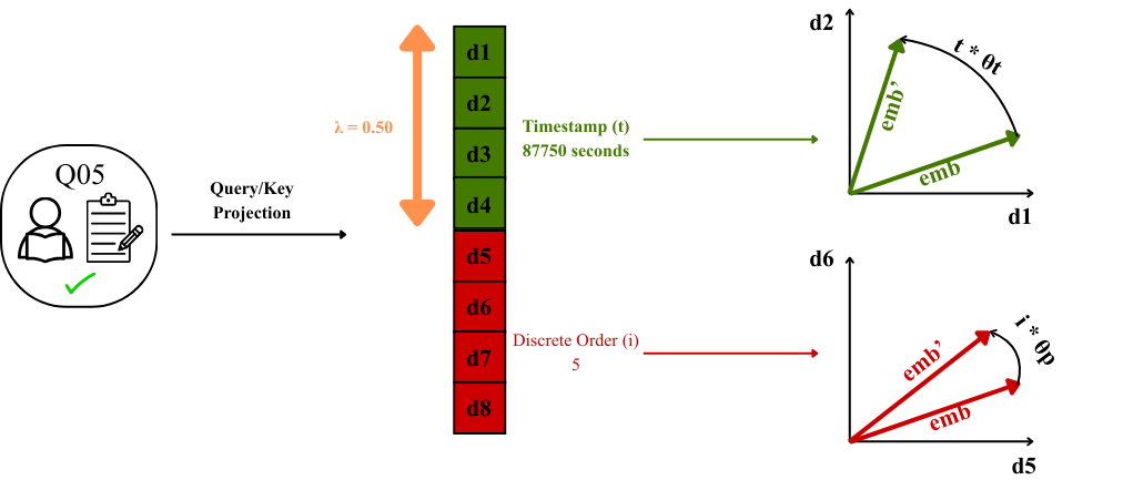
By defining position as a rotation in the latent space, the inner product naturally encodes the relative distance between interactions in terms of both discrete order (\(\Delta i\)) and continuous elapsed time (\(\Delta t\)). In our implementation, we define the temporal coordinate \(t\) as the absolute cumulative time (in seconds) relative to the student’s first interaction (\(t_0 = 0\)). Thus, while the model receives absolute timestamps as input, the rotation mechanism ensures that attention scores represent the relative time intervals between interactions. Figure 1 illustrates the alignment between these discrete order indices and the cumulative timestamps.
3.2 Separation Strategy
To effectively encode both discrete sequential order (\(i\)) and continuous elapsed time (\(t\)), we adopt the Split-by-Dimension strategy proposed by Wei et al. [27]. Wei et al. [27] suggested that integrating both signals into a single rotation plane can lead to destructive interference, in which conflicting phase shifts of time and order cancel each other out, destabilizing the attention mechanism. The Split-by-Dimension approach mitigates this by isolating the signals into orthogonal subspaces.
Formally, we partition the latent dimension \(d\) of each attention head into two disjoint sets of rotation planes: \(P\) (Order) and \(T\) (Time). We introduce a hyperparameter \(\lambda \in [0, 1]\) to control the time capacity ratio. It defines the proportion of dimensions allocated to temporal encoding.
Let \(\Psi _k \in \{0, 1\}\) be a gate function for the \(k\)-th rotation plane, determined by \(\lambda \):
The rotation angle \(\theta _k\) for a given interaction state \((i, t_i)\) is then defined as:
Here \(\omega _k^p\) and \(\omega _k^t\) are the angular frequencies derived from the geometric progression for order and time, respectively. \(\lambda =0.0\) implies a standard positional encoding (pure order), while \(\lambda =1.0\) results in a model driven purely by continuous time intervals. This mechanism allows the model to explicitly balance the inductive bias between sequence and time. Figure 2 illustrates this allocation.
3.3 Frequency Adjustment
To enable the model to capture both short-term immediate dependencies and long-term retention patterns, the angular frequencies of the rotation embeddings must be carefully calibrated. Following the methodology proposed by Wei et al. [27], we adopt a logarithmic frequency scale to ensure adequate resolution across different temporal scales.
The angular frequency \(\omega _k\) for the \(k\)-th rotation plane within a specific subspace is defined as:
Where \(N\) represents the number of rotation planes (2D subspaces) allocated to the specific feature (time or order) and \(k \in \{1, \dots , N\}\) is the index of the plane. The boundary frequencies, \(\omega _{max}\) and \(\omega _{min}\), are derived from the target wavelengths (periods) \(\beta \). Where \(\beta _{min}\) and \(\beta _{max}\) represent the lower and upper bounds of the resolution (wavelengths), respectively.
4. EXPERIMENTS
4.1 Datasets
|
Dataset |
Year(s) |
Interactions |
Students |
Questions |
KCs | Student Count with length \(> L\)
| ||||
|---|---|---|---|---|---|---|---|---|---|---|
| \(\mathbf {100}\) | \(\mathbf {200}\) | \(\mathbf {300}\) | \(\mathbf {400}\) | \(\mathbf {500}\) | ||||||
| Proprietary | 2023–2025 | 6,628,695 | 38,094 | 2,413 | 1,435 | 22,828 | 11,884 | 7,472 | 3,261 | 1,647 |
| EdNet | 2017–2019 | 95,293,926 | 784,309 | 13,169 | 188 | 112,558 | 76,718 | 59,108 | 48,087 | 40,260 |
| ASSIST2017 | 2004–2006 | 942,816 | 1,709 | 3,162 | 102 | 1,647 | 1,390 | 1,139 | 930 | 750 |
Previous works, such as Torralba and Efros [24] and Ben-David et al. [6], demonstrate that the intrinsic characteristics of each dataset, such as data distribution and collection biases, can significantly affect model performance. To mitigate performance gains arising from domain-specific overfitting, we selected three datasets with distinct characteristics for our evaluation.
The first is a Proprietary Dataset, a medium-sized corpus collected between 2023 and 2025 from response logs of students enrolled in various engineering courses within a Brazilian higher education institution. The second dataset is EdNet [10], a large-scale public benchmark containing interactions from Korean students collected between 2017 and 2019 for the TOEIC (Test of English for International Communication) exam. Finally, the third dataset is ASSISTments 2017 [4], a small dataset collected between 2004 and 2006 that comprises data from middle school students interacting with an Intelligent Tutoring System (ITS).
The combined use of these datasets allows us to evaluate model behavior across diverse scenarios, ranging from controlled educational environments to large-scale, real-world contexts. Table 1 summarizes the descriptive statistics for each dataset.
4.2 Data Partitioning and data processing
Yadav and Shukla [29] demonstrate that \(k\)-fold cross-validation typically offers the most robust evaluation metric. However, the authors also highlight the need to balance performance generalization with computational cost, which scales linearly with \(k\). Given the massive scale of the EdNet dataset and the requirement to perform grid searches for the TO-RoPE parameter \(\lambda \), strictly adhering to \(k\)-fold cross-validation would render the experimental timeline infeasible. For instance, training a single variation of the SAINT architecture on EdNet requires approximately 13 hours on an NVIDIA A100 GPU.
Due to these computational constraints, we adopted a student-level holdout strategy for the proprietary and EdNet datasets, using an 80/10/10 split (Train / Validation / Test). The partitioning was based on unique student identifiers, ensuring that students in the training set did not appear in the validation or test sets.
Regarding data processing, we addressed three critical scenarios:
- Sequence Splitting: To fully utilize extensive interaction histories, students with sequence lengths \(L > L_{window}\) were partitioned into \( N = L / L_{window}\) non-overlapping sub-sequences. This ensures that the model learns from the entire student’s trajectory, rather than just the initial interactions.
- Cold Start: Following the findings of Bhattacharjee and Wayllace [7], students with fewer than 5 interactions were removed from the datasets, as models lack sufficient context to make reliable predictions for such sparse histories.
- Padding: For sequences (or sub-sequences) with lengths \(L < L_{window}\), we appended padding tokens. These tokens are masked during training to prevent them from influencing the loss calculation.
In contrast, for the ASSISTments 2017 dataset, due to its smaller sample size, we adopted a nested evaluation strategy to ensure statistical robustness. First, we randomly selected 20% of the students as a test set. The remaining 80% of the data was used for 5-fold cross-validation to train the model and tune hyperparameters. This separation ensures that the final performance metrics are evaluated on a pristine set of unseen students.
4.3 RQ1: Length Extrapolation Analysis
To answer RQ1, we evaluated the capability of TO-RoPE to generalize to sequence lengths significantly longer than those observed during training by adopting a train-short, test-long protocol. The training and validation sets were divided into fixed windows of 100 interactions per student, following the configuration utilized by Choi et al. [9]. Interactions were classified chronologically by timestamp. During the testing phase, extrapolation capability was evaluated on windows of increasing lengths: 100, 200, 300, 400, and 500 interactions.
It is crucial to emphasize that the choice of a restricted training window (\(L=100\)) serves a dual purpose: it aligns with previous baselines and, more importantly, acts as a rigorous stress test for length generalization. Training on longer sequences (e.g., 500) and testing on similar lengths would fundamentally assess the model’s interpolation capabilities. By strictly limiting training to short sequences and evaluating on extended horizons, we effectively isolate and quantify the model’s capacity for real length extrapolation based on the learned geometric properties of the latent space.
Based on previous work [2, 20, 8], the Area Under the ROC Curve (AUC) was used as the primary performance metric. To ensure robustness, each model was executed with 5 different random seeds, and the results are reported as mean and standard deviation (\(\mu \pm \sigma \)). Due to a limited sample size (\(N=5\)) imposed by computational constraints, statistical significance was assessed using the Wilcoxon signed-rank test. We compared the baseline models (SAKT, SAINT) against their TO-RoPE variants. This non-parametric test was selected because it does not assume normality and is suitable for comparing classifiers across multiple runs [12]. Since our research hypothesis investigates the superiority of TO-RoPE over baselines, a one-sided test was adopted.
Additionally, to quantify stability, we report the slope coefficient (\(\alpha \)) from a linear regression of AUC values across different test window sizes. This metric indicates the trend of performance gain or degradation as the sequence length increases. For readability, the reported coefficients were scaled by a factor of 10000.
4.4 Analysis of Attention Dynamics
To assess RQ2, we investigated how the model interprets the temporal dimension, and to validate whether TO-RoPE effectively encodes continuous time as a geometric property, we conducted an empirical analysis of the attention weights. Our objective was to determine whether the incorporation of time (\(\lambda > 0\)) induces distinguishable attention patterns compared to purely ordinal baselines (\(\lambda = 0\)), specifically in terms of the modeling of knowledge decay.
We extracted the attention matrices \(A \in \mathbb {R}^{L \times L}\) from the inferences of the test set. To identify global patterns, we computed the mean attention scores averaged across all heads and layers for distinct configurations of \(\lambda \). These scores were then aggregated based on the time distance (\(\Delta t\)) between interactions \(i\) and \(j\). This aggregation strategy allows us to observe attention decay across varying temporal scales—ranging from immediate responses (seconds) to long-term retention intervals (weeks or months)—and to verify whether the model spontaneously learns to penalize older information based on elapsed time.
4.5 Hyperparameter Configuration
To ensure fair comparisons and reproducibility, hyperparameter tuning was tailored to each dataset’s scale. For large-scale datasets (EdNet and Proprietary), we adopted established configurations from the literature to manage computational costs. In contrast, for the smaller dataset ASSISTments2017, we performed a grid search to identify optimal settings.
Across all model architectures, batch sizes were determined by dataset scale to optimize throughput on the NVIDIA A100 GPU: we employed a batch size of 512 for the massive EdNet and 128 for both the Proprietary and ASSISTments2017 datasets.
For the SAINT architecture (and its TO-RoPE variants), we utilized the configuration proposed by Choi et al. [9] for EdNet and Proprietary datasets: latent dimension \(d=512\), \(h=8\) attention heads, \(L=4\) layers, and dropout \(p=0.1\). For ASSISTments2017, we searched over \(d \in \{64, 256, 512\}\), \(h \in \{4, 8\}\), \(L \in \{1, 2, 4\}\), and \(p \in \{0.05, 0.10, 0.20\}\).
For SAKT, we followed the recommendations of Pandey et al. [19] for large datasets, setting \(d=200\) and \(p=0.10\). For ASSISTments2017, we tuned the latent dimension over \(d \in \{50, 100, 200\}\).
For the AKT and LefoKT-AKT-NF baselines (with ALiBi), we strictly adhered to the hyperparameter settings described in their respective original papers [14, 5] for large-scale datasets: \(h=8\) heads, latent dimension \(d=512\), and dropout \(p=0.10\). However, for ASSISTments2017, we performed a specific grid search over the latent dimension \(d \in \{64, 256, 512\}\), number of heads \(h \in \{4, 8\}\), and dropout rates \(p \in \{0.05, 0.10, 0.20\}\).
All models were optimized using the Adam optimizer. We searched for the learning rate \(l_r \in \{1e^{-5}, 5e^{-5}, 1e^{-4}, 5e^{-4}, 1e^{-3}\}\), finding that \(l_r = 1e^{-4}\) is optimal for the majority configurations. Weights were initialized using the Xavier initialization scheme [15].
To avoid overfitting, we employed an early stopping mechanism with patience of 10 epochs, monitoring the AUC metric on the validation set with a minimum improvement delta of \(10^{-4}\). The maximum training duration was set at 50 epochs for SAINT-based models and 100 epochs for SAKT, AKT, and LefoKT.
Finally, for the Time Subspace, we set \(\beta _{min} = 1\) second across all datasets to capture fine-grained interactions. The upper bound \(\beta _{max}\) is set to the nearest power of 10 exceeding the maximum timestamp observed in each dataset, ensuring that the rotation mechanism covers the entire temporal span without aliasing. Table 2 details these dataset-specific bounds.
| Dataset | Max Time Observed (s) | \(\mathbf {\beta _{max}}\) (s) |
|---|---|---|
| Proprietary | \(\approx 7.80 \times 10^7\) | \(10^8\) |
| EdNet | \(\approx 8.17 \times 10^7\) | \(10^8\) |
| ASSIST2017 | \(\approx 5.02 \times 10^7\) | \(10^8\) |
For the Order Subspace, we fix \(\beta _{min} = 1\) and \(\beta _{max} = 500\). The latter corresponds to the maximum sequence length evaluated during our length extrapolation experiments, ensuring distinct positional signatures throughout the extended window.
5. RESULTS
5.1 RQ1: Length Extrapolation
| EdNet | ||||||
|---|---|---|---|---|---|---|
| Models | 100 | 200 | 300 | 400 | 500 | \(10000 \cdot \alpha \) |
| AKT | 0.7706 \(\pm \) 0.0003 | 0.7761 \(\pm \) 0.0004 | 0.7784 \(\pm \) 0.0006 | 0.7794 \(\pm \) 0.0005 | 0.7802 \(\pm \) 0.0006 | +0.22500 |
| LefoKT-AKT-NF + ALiBi | 0.7701 \(\pm \) 0.0004 | 0.7740 \(\pm \) 0.0005 | 0.7752 \(\pm \) 0.0005 | 0.7757 \(\pm \) 0.0006 | 0.7760 \(\pm \) 0.0006 | + 0.13499 |
| SAKT (baseline) | 0.7665 \(\pm \) 0.0001 | 0.7675 \(\pm \) 0.0002 | 0.7674 \(\pm \) 0.0002 | 0.7673 \(\pm \) 0.0003 | 0.7673 \(\pm \) 0.0003 | +0.01424 |
| SAKT + TOR (\(\lambda = 0.00\)) | 0.7649 \(\pm \) 0.0001 | 0.7683 \(\pm \) 0.0001* | 0.7694 \(\pm \) 0.0001* | 0.7698 \(\pm \) 0.0002* | 0.7700 \(\pm \) 0.0002* | +0.11869 |
| SAKT + TOR (\(\lambda = 0.50\)) | 0.7662 \(\pm \) 0.0001 | 0.7699 \(\pm \) 0.0001* | 0.7713 \(\pm \) 0.0002* | 0.7718 \(\pm \) 0.0002* | 0.7721 \(\pm \) 0.0003* | +0.13786 |
| SAKT + TOR (\(\lambda = 1.00\)) | 0.7666 \(\pm \) 0.0001 | 0.7709 \(\pm \) 0.0001* | 0.7726 \(\pm \) 0.0001* | 0.7734 \(\pm \) 0.0002* | 0.7739 \(\pm \) 0.0002* | +0.17094 |
| SAINT (baseline) | 0.7790 \(\pm \) 0.0004 | 0.7261 \(\pm \) 0.0004 | 0.7067 \(\pm \) 0.0006 | 0.6952 \(\pm \) 0.0006 | 0.6875 \(\pm \) 0.0008 | -2.13790 |
| SAINT + TOR (\(\lambda = 0.00\)) | 0.7761 \(\pm \) 0.0004 | 0.7806 \(\pm \) 0.0005* | 0.7808 \(\pm \) 0.0006* | 0.7801 \(\pm \) 0.0006* | 0.7795 \(\pm \) 0.0007* | +0.06258 |
| SAINT + TOR (\(\lambda = 0.50\)) | 0.7863 \(\pm \) 0.0004* | 0.7677 \(\pm \) 0.0005* | 0.7294 \(\pm \) 0.0007* | 0.7025 \(\pm \) 0.0009* | 0.6846 \(\pm \) 0.0012 | -2.69629 |
| SAINT + TOR (\(\lambda = 1.00\)) | 0.7866 \(\pm \) 0.0004* | 0.7939 \(\pm \) 0.0004* | 0.7976 \(\pm \) 0.0006* | 0.7999 \(\pm \) 0.0006* | 0.8016 \(\pm \) 0.0008* | +0.35792 |
| ASSISTments2017 | ||||||
| Models | 100 | 200 | 300 | 400 | 500 | \(10000 \cdot \alpha \) |
| AKT | 0.7382 \(\pm \) 0.0017 | 0.7388 \(\pm \) 0.0021 | 0.7359 \(\pm \) 0.0023 | 0.7329 \(\pm \) 0.0024 | 0.7312 \(\pm \) 0.0027 | -0.19915 |
| LefoKT-AKT-NF + ALiBi | 0.7466 \(\pm \) 0.0011 | 0.7492 \(\pm \) 0.0009 | 0.7502 \(\pm \) 0.0009 | 0.7508 \(\pm \) 0.0009 | 0.7512 \(\pm \) 0.0010 | +0.10822 |
| SAKT (baseline) | 0.7083 \(\pm \) 0.0011 | 0.7083 \(\pm \) 0.0016 | 0.7074 \(\pm \) 0.0011 | 0.7061 \(\pm \) 0.0011 | 0.7065 \(\pm \) 0.0009 | -0.05739 |
| SAKT + TOR (\(\lambda = 0.00\)) | 0.7248 \(\pm \) 0.0015* | 0.7230 \(\pm \) 0.0015* | 0.7200 \(\pm \) 0.0015* | 0.7177 \(\pm \) 0.0015* | 0.7167 \(\pm \) 0.0013* | -0.21541 |
| SAKT + TOR (\(\lambda = 0.50\)) | 0.7095 \(\pm \) 0.0016* | 0.7101 \(\pm \) 0.0017* | 0.7093 \(\pm \) 0.0016* | 0.7079 \(\pm \) 0.0015* | 0.7084 \(\pm \) 0.0013* | -0.04493 |
| SAKT + TOR (\(\lambda = 1.00\)) | 0.7068 \(\pm \) 0.0006 | 0.7084 \(\pm \) 0.0004* | 0.7078 \(\pm \) 0.0007* | 0.7071 \(\pm \) 0.0002* | 0.7072 \(\pm \) 0.0007* | -0.00451 |
| SAINT (baseline) | 0.7345 \(\pm \) 0.0015 | 0.6632 \(\pm \) 0.0027 | 0.6326 \(\pm \) 0.0026 | 0.6141 \(\pm \) 0.0027 | 0.6077 \(\pm \) 0.0034 | -3.02679 |
| SAINT + TOR (\(\lambda = 0.00\)) | 0.7580 \(\pm \) 0.0017* | 0.7603 \(\pm \) 0.0018* | 0.7607 \(\pm \) 0.0016* | 0.7546 \(\pm \) 0.0023* | 0.7331 \(\pm \) 0.0043* | -0.55579 |
| SAINT + TOR (\(\lambda = 0.50\)) | 0.7412 \(\pm \) 0.0046 | 0.7442 \(\pm \) 0.0047* | 0.7452 \(\pm \) 0.0048* | 0.7454 \(\pm \) 0.0049* | 0.7459 \(\pm \) 0.0049* | +0.10864 |
| SAINT + TOR (\(\lambda = 1.00\)) | 0.7189 \(\pm \) 0.0014 | 0.7169 \(\pm \) 0.0019* | 0.7160 \(\pm \) 0.0017* | 0.7141 \(\pm \) 0.0019* | 0.7137 \(\pm \) 0.0019* | -0.13214 |
| Proprietary Dataset
| ||||||
| Models | 100 | 200 | 300 | 400 | 500 | \(10000 \cdot \alpha \) |
| AKT | 0.8353 \(\pm \) 0.0006 | 0.8386 \(\pm \) 0.0007 | 0.8383 \(\pm \) 0.0008 | 0.8382 \(\pm \) 0.0009 | 0.8374 \(\pm \) 0.0009 | +0.03897 |
| LefoKT-AKT-NF + ALiBi | 0.8359 \(\pm \) 0.0002 | 0.8392 \(\pm \) 0.0002 | 0.8399 \(\pm \) 0.0002 | 0.8406 \(\pm \) 0.0002 | 0.8407 \(\pm \) 0.0002 | +0.10907 |
| SAKT (baseline) | 0.82891 \(\pm \) 0.0003 | 0.8134 \(\pm \) 0.0010 | 0.8057 \(\pm \) 0.0014 | 0.8001 \(\pm \) 0.0014 | 0.7973 \(\pm \) 0.0014 | -0.76963 |
| SAKT + TOR (\(\lambda = 0.00\)) | 0.8293 \(\pm \) 0.0001* | 0.8290 \(\pm \) 0.0002* | 0.8275 \(\pm \) 0.0002* | 0.8262 \(\pm \) 0.0001* | 0.8250 \(\pm \) 0.0002* | -0.11241 |
| SAKT + TOR (\(\lambda = 0.50\)) | 0.8352 \(\pm \) 0.0002* | 0.8353 \(\pm \) 0.0002* | 0.8336 \(\pm \) 0.0003* | 0.8323 \(\pm \) 0.0003* | 0.8313 \(\pm \) 0.0003* | -0.10678 |
| SAKT + TOR (\(\lambda = 1.00\)) | 0.8341 \(\pm \) 0.0004* | 0.8342 \(\pm \) 0.0003* | 0.8329 \(\pm \) 0.0003* | 0.8318 \(\pm \) 0.0002* | 0.8310 \(\pm \) 0.0002* | -0.08638 |
| SAINT (baseline) | 0.8371 \(\pm \) 0.0005 | 0.7834 \(\pm \) 0.0022 | 0.7651 \(\pm \) 0.0029 | 0.7537 \(\pm \) 0.0034 | 0.7491 \(\pm \) 0.0037 | -2.05643 |
| SAINT + TOR (\(\lambda = 0.00\)) | 0.8485 \(\pm \) 0.0003* | 0.8497 \(\pm \) 0.0008* | 0.8456 \(\pm \) 0.0019* | 0.8421 \(\pm \) 0.0024* | 0.8399 \(\pm \) 0.0026* | -0.24775 |
| SAINT + TOR (\(\lambda = 0.50\)) | 0.8513 \(\pm \) 0.0004* | 0.8543 \(\pm \) 0.0009* | 0.8518 \(\pm \) 0.0038* | 0.8491 \(\pm \) 0.0057* | 0.8472 \(\pm \) 0.0065* | -0.13354 |
| SAINT + TOR (\(\lambda = 1.00\)) | 0.8484 \(\pm \) 0.0005* | 0.8518 \(\pm \) 0.0005* | 0.8522 \(\pm \) 0.0006* | 0.8521 \(\pm \) 0.0006* | 0.8516 \(\pm \) 0.0006* | +0.06858 |
Note: Values represent mean \(\pm \) std. dev. over 5 independent runs. * denotes statistical significance (\(p < 0.05\)) compared to the baseline (one-sided Wilcoxon signed-rank test). Bold values indicate best performance per window. \(\alpha \): slope of linear regression (scaled by 10000 to ease legibility) over window sizes (stability metric).
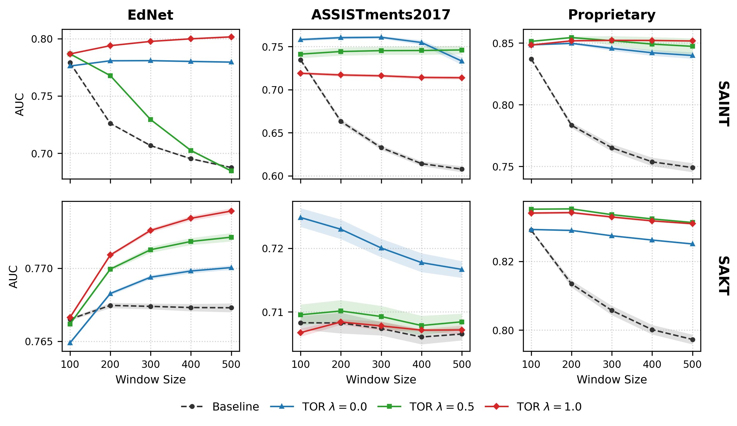
The initial results present the length extrapolation capabilities of the TO-RoPE models compared to baselines, with performance trajectories visualized in Figure 3 and quantitative metrics detailed in Table 3.
In the EdNet dataset, the SAINT + TO-RoPE configuration (\(\lambda = 1.00\)) achieved the highest AUC values across all test windows, distinguishing itself by a growing performance trend as the sequence extended (\(10000 \cdot \alpha = +0.35792\)). In contrast, both the SAINT baseline and the variation with \(\lambda = 0.50\) exhibited a performance collapse, with sharp AUC drops starting from the first extrapolation window. Regarding SAKT, the time-focused variation (\(\lambda = 1.00\)) led across all window lengths; however, the gains were significantly less expressive than those observed in SAINT. Variations with \(\lambda = 0.50\) and \(\lambda = 0.00\) demonstrated intermediate performance, while the baseline remained stable but with AUC scores inferior to all rotation-based variations from 200 interactions onward. Models such as AKT and LefoKT maintained positive slopes and outperformed SAKT variants, but did not reach the performance level of SAINT + TO-RoPE (\(\lambda = 1.00\)).
For ASSISTments2017, the SAINT + TO-RoPE variation with \(\lambda = 0.00\) (purely order-based) presented the best performance in windows from 100 to 400 interactions. At the limit of 500 interactions, the LefoKT-AKT-NF + ALiBi model obtained the superior result. Contrary to trends in EdNet, the temporal variation (\(\lambda = 1.00\)) in SAINT underperformed, yielding consistently lower results than the order-based variants. The SAINT baseline showed an acute performance decline in the extended windows. In the SAKT model, the variation \(\lambda = 0.00\) was the most effective, leading both in absolute AUC values and stability metrics, whereas temporal variation led to performance degradation. The AKT outperformed all SAKT variants in this dataset, though it remained inferior to SAINT.
Results on the Proprietary dataset exhibited mixed behavior. The SAINT + TO-RoPE configuration with \(\lambda = 0.50\) led in the initial windows of 100 and 200 interactions, while the purely time-based version (\(\lambda = 1.00\)) obtained the best results in the 300, 400, and 500 windows, also registering the highest stability (\(\alpha \)) among SAINT-based models. In the case of SAKT, the hybrid model (\(\lambda = 0.50\)) was superior to the other variations in all the extensions tested. The baselines for both models (SAINT and SAKT) suffered significant performance drops. Finally, the AKT and LefoKT-AKT-NF + ALiBi models demonstrated competitiveness, maintaining positive stability slopes, with LefoKT reaching the highest overall stability recorded for this dataset (\(10000 \cdot \alpha = +0.10907\)).
Additionally, we computed the average ordinal distance (\(\overline {\Delta O}\)) within each bucket to understand the density of sessions. These statistics are summarized in Table 4.
| First int. | Hour | Day | Week | Month | > 1 Month
| ||||||
|---|---|---|---|---|---|---|---|---|---|---|---|
| Dataset | % | % | \(\overline {\Delta O}\) | % | \(\overline {\Delta O}\) | % | \(\overline {\Delta O}\) | % | \(\overline {\Delta O}\) | % | \(\overline {\Delta O}\) |
| Proprietary | 33.84% | 28.44% | 6.36 | 3.64% | 12.91 | 9.84% | 15.88 | 13.64% | 22.42 | 10.60% | 89.17 |
| EdNet | 16.44% | 36.02% | 7.71 | 14.25% | 49.35 | 21.37% | 106.07 | 7.92% | 244.89 | 4.00% | 379.29 |
| ASSIST2017 | 7.55% | 82.19% | 3.24 | 0.21% | 68.05 | 0.49% | 64.19 | 3.87% | 60.58 | 5.68% | 158.86 |
5.2 RQ2: Temporal Attention Dynamics
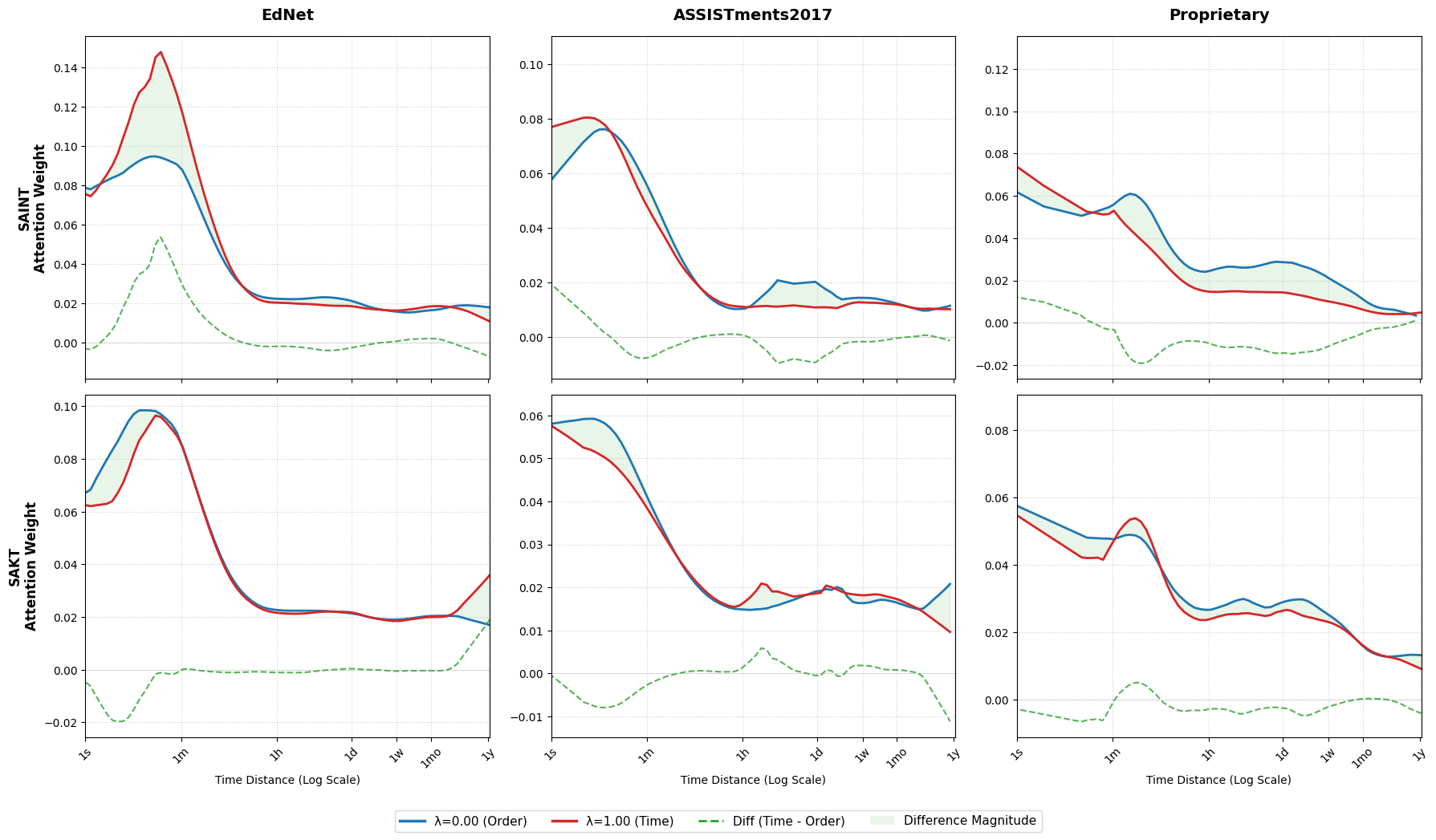
Figure 4 illustrates the attention decay patterns as a function of the temporal distance between interactions. A prominent feature is observed in the EdNet dataset with the SAINT architecture. The temporal model (\(\lambda =1.00\)) concentrates significantly higher attention weights on short-term interactions (\(1s \le \Delta t \le 1h\)) compared to the ordinal baseline. As the time interval extends beyond 1 hour, both curves converge to similar low-magnitude values. On the other hand, for the SAKT architecture on EdNet, a divergent pattern emerges: the ordinal model (\(\lambda =0.00\)) assigns higher attention to immediate interactions (\(1s \le \Delta t \le 1min\)) than the temporal variant. For longer intervals (\(1mo \le \Delta t \le 1y\)), the difference between the two configurations stabilizes near zero.
Regarding ASSISTments2017, while there are differences between the ordinal and temporal attention distributions for both SAINT and SAKT in the short-to medium term, the magnitude of these deviations is less pronounced than those observed in the EdNet/SAINT scenario.
Finally, in the Proprietary dataset, the SAINT model with temporal encoding (\(\lambda =1.00\)) exhibits a dual behavior: it assigns higher weights to very short-term interactions while systematically suppressing attention to distant past interactions more aggressively than the ordinal model. A similar trend is observed in SAKT, except that in the short term, the ordinal model predominates.
Despite these architecture-specific variations, a consistent global pattern is evident across all models and datasets: attention scores exhibit a natural decay as the temporal interval increases. This decay is notably sharper for EdNet and ASSISTments2017, whereas the Proprietary dataset displays a smoother, more gradual decline.
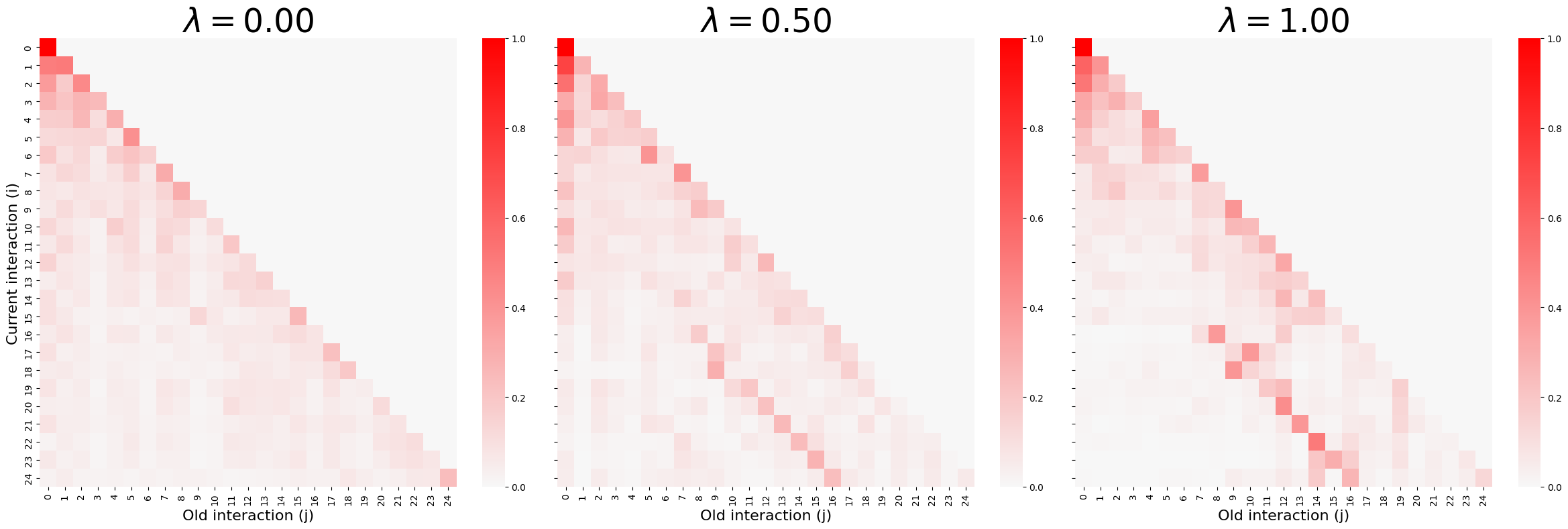
In an order-based model, such as SAINT + TO-RoPe (\(\lambda = 0.00\)), an item 20 steps ago is treated as a distant context. However, TO-RoPE (\(\lambda =1.00\)) correctly identifies that these 20 items occurred on the same day, indicating a learning burst. This explains the attention patterns observed in Figure 5:
- Order-based (\(\lambda =0.00\)): Attention is strictly diagonal, suffering from recency bias.
- Time-based (\(\lambda > 0\)): The attention mechanism diffuses off the diagonal, successfully attending to temporally clustered interactions that are ordinally distant.
This ability to compress bursts (treating them as simultaneous) while respecting long-term gaps allows the model to better capture complex temporal patterns, driving the superior extrapolation results seen in EdNet.
The interplay between time and order is most nuanced in the Proprietary dataset, where the hybrid configuration (\(\lambda =0.50\)) often yields superior stability. Unlike the self-paced nature of EdNet, higher education engineering courses follow a structured curriculum where sequential prerequisites are strictly enforced (favoring Order). However, students frequently engage in “cramming” sessions before exams, generating high-frequency bursts (favoring Time). A balanced \(\lambda \) allows the model to simultaneously respect the curricular sequence while geometrically compressing these intensive study sessions. This suggests that TO-RoPE is not a one-size-fits-all solution, but a flexible framework adaptable to the specific pedagogical design of the learning environment.
6. DISCUSSION
The inclusion of TO-RoPE significantly enhances length extrapolation capabilities, but the magnitude of these gains is highly sensitive to the dataset’s characteristics. To deconstruct these performance variations, we analyzed the temporal distribution of the interactions. We aggregated interactions into time buckets based on the elapsed time since the student last engaged with the same KC.
Beyond specific dataset characteristics, the fundamental success of TO-RoPE in length extrapolation (RQ1) stems from the geometric property of translation invariance. Standard models fail because the absolute embeddings (\(P_i\)) learned for positions \(i \in [0, L_{train}]\) are undefined or semantically meaningless for \(i > L_{train}\). In contrast, TO-RoPE encodes the relative distance between interactions. For the attention mechanism, a temporal gap of \(\Delta t = 1\) hours possesses the same geometric representation, whether it occurs at the beginning of a course or after thousands of interactions. This ensures that predictive stability is maintained indefinitely, effectively decoupling the model’s context capacity from the fixed window sizes used during training.
The poor performance of the time-only variant (\(\lambda =1.00\)) in ASSISTments2017 can be attributed to a low temporal signal-to-noise ratio. As shown in Table 4, nearly 90% of all interactions in this dataset occur within the first hour of contact with a KC. In such a highly dense short-term environment, the continuous timestamp provides negligible additional information beyond the discrete sequence order. Consequently, dedicating latent dimensions to time rotation (\(\lambda > 0\)) likely displaces valuable ordinal capacity without providing a discriminative signal, effectively acting as noise that degrades performance.
In contrast, EdNet exhibits a heavy-tailed distribution with a significant interaction volume spread across Days (14.25%), Weeks (21.37%), and even Months (7.92%). The table reveals a discrepancy between ordinal and temporal proximity: interactions within the same "Day" or "Week" bucket often have large ordinal distances (\(\overline {\Delta O} \approx 49\) and 106, respectively).
Based on the findings regarding RQ2, incorporating continuous time as a geometric property alters the model’s attention dynamics by decoupling ordinal distance from temporal distance. The empirical analysis, particularly on the EdNet dataset, reveals that purely order-based models exhibit a strict diagonal focus driven by recency bias—treating a prerequisite 20 steps ago as a distant context regardless of how quickly those interactions occurred. In contrast, the TO-ROPE mechanism effectively compresses rapid-fire bursts of activity. By geometrically recognizing that high-frequency sequences occur within a negligible time window despite their ordinal length, the model spontaneously diffuses attention across these clusters. This confirms that geometric encoding enables the attention mechanism to filter out noise from high-volume interaction bursts and to perceive the cognitive density of a learning session, rather than simply counting steps.
Furthermore, the study demonstrates that interpretable knowledge decay patterns emerge naturally from these geometric rotations, without the need for the handcrafted, monotonic penalty functions used in prior architectures such as AKT or LefoKT. While the attention weights exhibit a spontaneous forgetting curve as the temporal gap increases, the rotation mechanism preserves the norm of the latent vectors rather than imposing bias. This structural property enables the model to attenuate outdated information while still retaining the capacity to revisit and address distant but semantically critical prerequisites when vector alignment is strong. This finding suggests that geometric encoding offers a superior inductive bias, balancing the natural tendency to forget with the ability to recall long-term dependencies when the specific learning context demands it.
This research advances KT research by establishing that student learning trajectories are better modeled as continuous geometric paths in a latent space than as rigid, discrete sequences. The study shows that critical cognitive phenomena, such as memory decay and the spacing effect, can emerge from the relative rotation of the query and key vectors without the need for handcrafted penalty functions or additive biases. This shift challenges the prevailing reliance on absolute positional embeddings by proposing a unified framework that treats discrete order and continuous time as orthogonal yet complementary geometric dimensions.
The practical implications of this study extend to both the computational scalability of lifelong learning systems and the quality of personalized educational interventions. From a systems perspective, the findings demonstrate that models can be trained on efficient, truncated interaction windows (e.g., 100 steps) while maintaining predictive stability over substantially longer student histories (up to 500 steps). This decoupling of training context from inference capacity prevents the performance collapse typical of standard Transformer architectures, allowing platforms to deploy robust models without incurring prohibitive computational costs. Consequently, this framework enables more stable performance predictions for learners with extensive interaction histories, which is essential for reliably tracking student progress across an entire course or even years of study. Furthermore, by accurately capturing natural memory decay, TO-RoPE empowers adaptive systems to deliver smarter, timely interventions, such as scheduling targeted reviews or spaced repetitions based on a student’s probability to forget a concept.
7. LIMITATIONS AND FUTURE WORKS
Despite not changing the time complexity of the main attention mechanism, incorporating TO-RoPE adds a computational overhead when searching for the optimal time-capacity ratio hyperparameter (\(\lambda \)). Additionally, the model’s effectiveness depends on the dataset’s temporal signal-to-noise ratio. In environments with low temporal variance, such as ASSISTments2017, allocating dimensions to time can degrade performance by displacing valuable ordinal information. To address these challenges, future research could use interpretability techniques, such as Attention Rollout, to analyze how individual heads specialize in capturing either short-term bursts or long-term decay.
In terms of baselines, we also recommend expanding the comparative analysis to other time-aware models, such as DKT-Forget [18], Deep Graph Memory Network (DGMN) [1], Long Sequence Temporal Knowledge Tracing (LSTKT) [13], and HawkesKT [26], to evaluate how well TO-RoPE performs compared to these distinct approaches. Furthermore, this framework could be expanded to diverse educational domains, such as Law and Humanities, to investigate how different knowledge structures interact with geometric temporal properties.
8. ACKNOWLEDGMENTS
This research was partially supported by the Brazilian National Council for Scientific and Technological Development - CNPq (301415/2025-0).
9. REFERENCES
- G. Abdelrahman and Q. Wang. Deep graph memory networks for forgetting-robust knowledge tracing. IEEE Transactions on Knowledge and Data Engineering, 35(8):7844–7855, 2022.
- G. Abdelrahman, Q. Wang, and B. Nunes. Knowledge tracing: A survey. ACM Comput. Surv., 55(11), Feb. 2023.
- I. Ahmad, S. Sharma, R. Singh, A. Gehlot, N. Priyadarshi, and B. Twala. Mooc 5.0: A roadmap to the future of learning. Sustainability, 14(18), 2022.
- ASSISTments. Assistments data mining competition 2017 dataset. https://sites.google.com/view/assistmentsdatamining/dataset, 2017. Accessed: [20/01/2026].
- Y. Bai, X. Li, Z. Liu, Y. Huang, M. Tian, and W. Luo. Rethinking and improving student learning and forgetting processes for attention based knowledge tracing models. Proceedings of the AAAI Conference on Artificial Intelligence, 39(27):27822–27830, Apr. 2025.
- S. Ben-David, J. Blitzer, K. Crammer, A. Kulesza, F. Pereira, and J. W. Vaughan. A theory of learning from different domains. Machine learning, 79(1):151–175, 2010.
- I. Bhattacharjee and C. Wayllace. Cold start problem: An experimental study of knowledge tracing models with new students. In International Conference on Artificial Intelligence in Education, pages 425–432. Springer, 2025.
- M. Cao, P. I. P. Jr., W. Chu, and L. Zhang. Integrating attentional factors and spacing in logistic knowledge tracing models to explore the impact of train-ing sequences on category learning. pages 526–532, July 2024.
- Y. Choi, Y. Lee, J. Cho, J. Baek, B. Kim, Y. Cha, D. Shin, C. Bae, and J. Heo. Towards an appropriate query, key, and value computation for knowledge tracing. In Proceedings of the Seventh ACM Conference on Learning @ Scale, L@S ’20, page 341–344, New York, NY, USA, 2020. Association for Computing Machinery.
- Y. Choi, Y. Lee, D. Shin, J. Cho, S. Park, S. Lee, J. Baek, C. Bae, B. Kim, and J. Heo. Ednet: A large-scale hierarchical dataset in education. In International conference on artificial intelligence in education, pages 69–73. Springer, 2020.
- Y. Cui, Z. Ma, L. Wang, A. Yang, Q. Liu, S. Kong, and H. Wang. A survey on big data-enabled innovative online education systems during the covid-19 pandemic. Journal of Innovation Knowledge, 8(1):100295, 2023.
- J. Demšar. Statistical comparisons of classifiers over multiple data sets. Journal of Machine learning research, 7(Jan):1–30, 2006.
- A. Gao and Z. Liu. Long sequence temporal knowledge tracing for student performance prediction via integrating lstm and informer. PLoS One, 20(9):e0330433, 2025.
- A. Ghosh, N. Heffernan, and A. S. Lan. Context-aware attentive knowledge tracing, 2020.
- X. Glorot and Y. Bengio. Understanding the difficulty of training deep feedforward neural networks. In Proceedings of the thirteenth international conference on artificial intelligence and statistics, pages 249–256. JMLR Workshop and Conference Proceedings, 2010.
- K. Hong, K. Karbasi, and G. Pottie. Extracting causal relations in deep knowledge tracing. pages 586–591, July 2025.
- X. Li, Y. Bai, T. Guo, Z. Liu, Y. Huang, X. Zhao, F. Xia, W. Luo, and J. Weng. Enhancing length generalization for attention based knowledge tracing models with linear biases. In Proceedings of the thirty-third international joint conference on artificial intelligence (IJCAI-24), pages 5918–5926, 2024.
- K. Nagatani, Q. Zhang, M. Sato, Y.-Y. Chen, F. Chen, and T. Ohkuma. Augmenting knowledge tracing by considering forgetting behavior. In The world wide web conference, pages 3101–3107, 2019.
- S. Pandey and G. Karypis. A self-attentive model for knowledge tracing, 2019.
- M. Pankiewicz, Y. Shi, and R. S. Baker. srcml-dkt: Enhancing deep knowledge tracing with robust code representations from srcml. In C. Mills, G. Alexandron, D. Taibi, G. L. Bosco, and L. Paquette, editors, Proceedings of the 18th International Conference on Educational Data Mining, pages 541–548. International Educational Data Mining Society, July 2025.
- C. Piech, J. Spencer, J. Huang, S. Ganguli, M. Sahami, L. Guibas, and J. Sohl-Dickstein. Deep knowledge tracing, 2015.
- J. Su, M. Ahmed, Y. Lu, S. Pan, W. Bo, and Y. Liu. Roformer: Enhanced transformer with rotary position embedding. Neurocomputing, 568:127063, 2024.
- A. C. Topuz, E. Saka, Ö. F. Fatsa, et al. Emerging trends of online assessment systems in the emergency remote teaching period. Smart Learning Environments, 9(1):17, 2022.
- A. Torralba and A. A. Efros. Unbiased look at dataset bias. In CVPR 2011, pages 1521–1528. IEEE, 2011.
- A. Vaswani, N. Shazeer, N. Parmar, J. Uszkoreit, L. Jones, A. N. Gomez, L. Kaiser, and I. Polosukhin. Attention is all you need, 2023.
- C. Wang, W. Ma, M. Zhang, C. Lv, F. Wan, H. Lin, T. Tang, Y. Liu, and S. Ma. Temporal cross-effects in knowledge tracing. In Proceedings of the 14th ACM international conference on web search and data mining, pages 517–525, 2021.
- X. Wei, J. Wu, D. Yi, R. Shirkavand, and M. Gong. Rotate both ways: Time-and-order rope for generative recommendation, 2025.
- Y. Wu, M. Arevalillo-Herráez, and D. Arnau. A study of the influence of the attention mechanism on knowledge tracing. In International Conference on Artificial Intelligence in Education, pages 462–469. Springer, 2025.
- S. Yadav and S. Shukla. Analysis of k-fold cross-validation over hold-out validation on colossal datasets for quality classification. In 2016 IEEE 6th International conference on advanced computing (IACC), pages 78–83. IEEE, 2016.
- B. Yamkovenko, C. Hogg, M. Miller-Vedam, P. Grimaldi, and W. Wells. Practical evaluation of deep knowledge tracing models for use in learning platforms. pages 673–679, July 2025.
© 2026 Copyright is held by the author(s). This work is distributed under the Creative Commons Attribution-NonCommercial-NoDerivatives 4.0 International (CC BY-NC-ND 4.0) license.