ABSTRACT
Learning analytics (LA) and educational data mining offer powerful ways to study self-regulated learning (SRL), but privacy constraints often restrict access to authentic learner data, limiting reproducibility and collaboration. Synthetic data generation (SDG) provides a promising approach by preserving statistical properties of real data while mitigating privacy risks. This study evaluates synthetic SRL datasets along three dimensions: their resemblance to real data, their utility for predicting student success, and their capacity to reproduce prior explainable AI (XAI) findings. Results show that BayesNet-based SDG most effectively approximated real data and enabled predictive models that in some cases outperformed those trained on authentic data. Synthetic datasets also replicated XAI stability metrics from prior work, though contextual effects such as those linked to COVID-19 remained difficult to capture. Grounded in SRL theory, this study demonstrates both the promise and limitations of SDGs and contributes a publicly available multi-dimensional dataset for open LA research.
Keywords
1. INTRODUCTION
Advancements in data collection and processing within the educational domain have given rise to the field of learning analytics (LA), which aims to optimize learning processes and environments in a data-driven manner [39]. Self-regulated learning (SRL), which has been shown to be important for student success [53, 54], can be studied by processing the data traces left by students interacting and engaging with online environments [49]. The potential of LA data to capture SRL is well-recognized [48]. Additionally, Educational Data Mining (EDM) can help to operationalize SRL constructs, to investigate the relationships between these constructs, to model and understand student learning trajectories, and to clarify how far we can trust conclusions and findings [49]. LA trace data has been shown to be most informative for predicting student success when higher level study indicators are generated from the highly granular trace data [17]. Dashboards and other LA tools that provide support for SRL aspects such as goal setting, monitoring, and self-reflection have been shown capable of positively influencing learning motivation and engagement, on condition that tools explicitly link their functionalities to SRL theories and constructs [55], and are grounded in educational theories [30, 46]. Extracting meaningful SRL indicators from trace data using EDM is an important prerequisite for providing effective LA tool support.
The use of actual, real-world trace data to support LA and evaluate SRL effectiveness is hindered by ethical and privacy concerns [43]. Access to real learning data is often restricted due to privacy regulations such as the GDPR in Europe, as well as institutional policies on processing student data – where data collection primarily serves the organization and administration of education. These restrictions complicate open science and collaborative research. One promising solution is the generation and use of synthetic data, which is a class of techniques that preserve the statistical properties of the original datasets while reducing the risks of information disclosure, re-identification or reconstruction [4]. This promise is amplified by recent advances in GenAI techniques capable of generating structured tabular datasets [18]. The synthetic data generation approach is especially valuable in large educational information systems composed of multiple services owned by different stakeholders, where data sharing is inherently challenging. By enabling safer data exchange, synthetic data can facilitate faster system development and testing, promote collaboration, and support broader adoption of LA [4].
In this paper, we examine the extent to which artificially generated data on learners’ self-regulation (1) resembles real data, (2) can be leveraged to predict student success, and (3) enables the replication of prior studies on explainable AI (XAI) in LA. Our primary contribution is an in-depth comparative evaluation of the potential of synthetic datasets within the broader LA research domain, along with an analysis of their use in the context of XAI stability. In addition, we provide a synthetic dataset that addresses the scarcity of publicly available LA data. To support the link with SRL, we focus on a dataset constituted of SRL indicators, next to outcome data. This dataset is multi-dimensional, spanning multiple courses and academic years, and thus supports out-of-sample validation across both contexts and time.
This paper is organized as follows. Section 2 discusses related work, identifies research gaps and states the research questions. Section 3 details the study’s methodology, including descriptions of the data and synthetic data generators, as well as the analysis setup. Section 4 reports the findings and Section 5 provides a broader discussion of the results, including the limitations and directions for future work. Finally, Section 6 summarizes the main contributions.
2. RELATED WORK
2.1 Synthetic Data Generation in LA
Privacy and confidentiality concerns have driven the adoption of synthetic data generators (SDGs). These tools are capable of learning the characteristics of real datasets to produce synthetic data with similar statistical properties [51]. Several publicly available SDG libraries exist, including Synthcity [35] and the Synthetic Data Vault (SDV) [33].
Statistical techniques such as Markov models or Bayesian networks (BayesNet) are widely used for synthetic data generation in education. Flanagan et al. [11] investigated the effectiveness of using synthetic educational data for real-world scenarios involving data sharing with third parties. The synthetic data was generated using a first-order Markov model trained on real interaction data from a digital material reading system, where learner actions were modeled as states and transition probabilities were learned from the original dataset. To evaluate the quality of the synthetic data, models were trained on it to predict academic achievement and then tested on real, private data. Several of these models showed significantly lower performance when applied to the non-synthetic datasets, indicating limitations in the utility of the synthetic data. On the other hand, the experiment of Dorodchi et al. [9] generated synthetic educational data using Bayesian networks and the models trained on synthetic data performed similarly to those trained on real data in benchmark tasks, suggesting synthetic data can be a viable alternative for algorithm development in LA.
In many machine learning (ML) studies, statistical methods are frequently benchmarked against more complex deep learning models (e.g., [14]), and SDG is no exception. Zhan et al. [51] evaluated four SDG techniques – GaussianCopula, CTGAN, CopulaGAN, and TVAE – for their ability to generate high-quality synthetic student data. Their evaluation followed a two-step process: (1) comparing the distributional similarity between synthetic and original datasets; and (2) assessing the utility of the synthetic data in LA tasks such as regression and classification. The results indicated that GaussianCopula and TVAE performed best, producing synthetic data that both closely mirrored the original distributions and enabled strong performance on downstream tasks. Expanding on this, Liu et al. [25] conducted a comparative analysis of SDGs in LA – including Gaussian Multivariate (GM), Gaussian Copula, and CTGAN – using metrics for similarity, utility, and privacy. While GM performed well in terms of utility, it fell short in privacy protection: the close resemblance between GM-generated synthetic data and the real data increases the risk of exposing sensitive information. In contrast, Gaussian Copula offered the most balanced performance across all three dimensions, making it the preferred choice for LA tasks.
The emergence of large language models (LLMs) has spurred their adoption in the domain of synthetic data generation. In addition to the widely used CTGAN model, Khalil et al. [18] employed three different LLMs to generate synthetic tabular data. The resulting datasets exhibited strong alignment with real-world data, particularly in terms of statistical similarity. Their findings showed that CTGAN achieved performance comparable to that of the LLM-based approaches, with both CTGAN and DialoGPT emerging as the top performers overall.
Liu et al. [24] investigated the trade-off between privacy and fairness in synthetic data generation, evaluating both GAN-based models and LLMs using standard ML algorithms as well as fairness-aware methods. In LA, privacy concerns center on obtaining learners’ consent for data collection and preventing harm from data sharing, while fairness focuses on avoiding the reinforcement of existing societal biases against minority groups in LA solutions. Their study found that the DECAF model achieved the best overall balance between privacy and fairness, albeit at the cost of the lowest utility performance. For use cases where privacy is the primary concern, ADSGAN was identified as the most suitable option. Table 1 summarizes the abovementioned studies on investigating the performance reported for existing SDGs.
2.2 Stability Analysis in Learning Analytics
One of the key downstream tasks in LA is predicting student success using ML models trained on learning indicators derived from detailed study activity data, in alignment with SRL theory [17]. The insights generated by these models can support feedback provision, such as personalized study advice and timely interventions. However, real-time study data is not always accessible due to privacy regulations (e.g., GDPR), making models trained on historical data the default choice for many LA practitioners. Consequently, the usefulness of these models depends on their stability across academic years and their ability to adapt to changing contexts [31].
Tempelaar et al. [41] investigated the stability and sensitivity of LA prediction models across different student cohorts and instructional designs by using linear regression models. They find that models are stable when the instructional design remains unchanged, maintaining similar predictors and accuracy. However, when the course design changes, the models show sensitivity, hence affecting model stability. Saqr et al. [38] perform a single-paper meta-analysis (using correlation analysis for each individual analysis) to identify which commonly used LA indicators reliably generalize across course runs, reporting total activity and forum participation as the most consistently portable predictors across similar course contexts.
Tiukhova et al. [44] extended prior work by evaluating the stability of LA models over time and across student cohorts, employing both statistical and ML techniques alongside XAI methods. By integrating XAI, they introduced an important explainability dimension into model stability analysis. XAI encompasses a variety of approaches that make AI models “more intelligible to humans by providing explanations” [15]. In educational settings, explainable AI (XAI-ED) has been conceptualized as a structured framework that addresses six interrelated dimensions – stakeholders, benefits, explanation methods, model types, human-centered interface design, and explanation-specific pitfalls – in order to meet the unique needs of educational contexts [19].
Building on this foundation, Tiukhova et al. [44] combined concept and prediction drift analysis with explainability as a diagnostic tool. They demonstrated how feature-importance rankings generated by SHAP [29] can be used to assess whether model explanations remain consistent across cohorts. They show that explainability can enrich stability analysis by complementing traditional techniques and uncovering new insights: SHAP not only clarified model predictions but also functioned as a diagnostic tool for evaluating global model stability across contexts. The authors conclude that LA models should be updated, as only general engagement metrics consistently remain reliable [44].
2.3 Research gap and research questions
Evaluating reproducibility is a key requirement for ensuring generalizable outcomes in both LA and SRL research. However, it has not been systematically explored yet in the context of SDGs. This paper addresses this gap by specifically examining the reproducibility of existing LA research findings on model stability across cohorts and over time, i.e., whether models and their explanations remain consistent across time and cohorts [44] when synthetic data is used for these models. Crucially, the artificially generated data is based on a dataset containing meaningful SRL indicators to ensure that its educational relevance and interpretability are preserved. In addition, it is essential to compare the reproducibility-oriented utility of SDGs with more conventional measures – statistical resemblance and predictive performance – to determine whether commonly used evaluation criteria truly reflect the capacity of synthetic data to support valid and transferable LA research conclusions. The research therefore first assesses the quality of the synthetic data along the state of the art dimensions of statistical resemblance (RQ1) and prediction performance (RQ2). It then advances the state of the art by investigating the reproducability of the stability analysis (RQ3) and verifying the alignment to the results of RQ1 and RQ2. The RQs are therefore as follows:
- RQ1 Statistical resemblance
- To what extent does synthetic data resemble real data in terms of distributional similarity, and which SDG algorithms produce the most realistic distributions?
- RQ2 Prediction utility
- How effectively can synthetic data be used for student success prediction, and which SDG algorithms yield a dataset that can be used to train the models with the highest prediction performance when applied to the real data?
- RQ3 Replication utility
- To what extent can synthetic data be used to replicate existing research going beyond predictions – specifically, the stability analysis conducted by Tiukhova et al. [44] – and which SDG algorithms produce a dataset allowing for the highest degree of reproducibility of the stability analysis?
3. METHODOLOGY
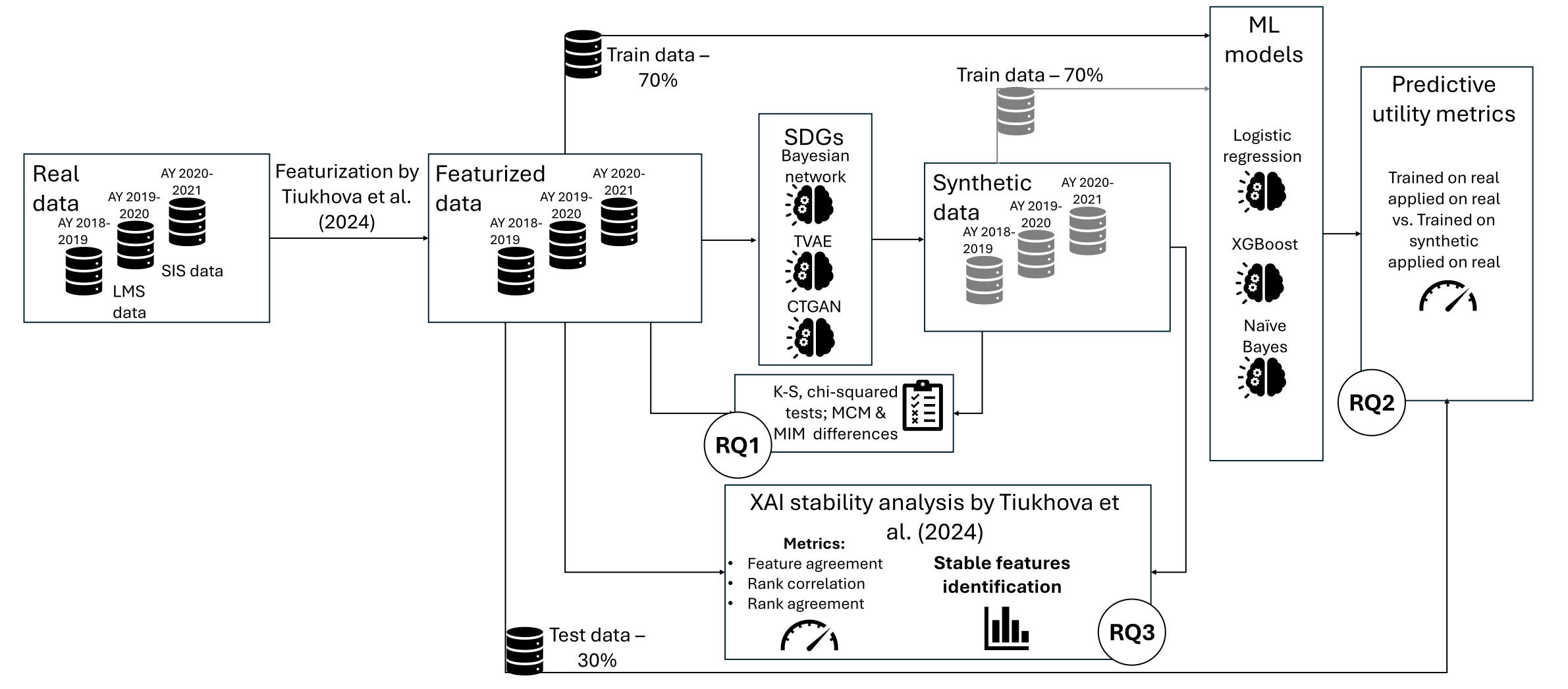
We first discuss data collection and feature engineering activities, after which we detail the selected SDGs for this study. Then, we elaborate on the main methodology to assess (i) statistical resemblance, (ii) prediction utility, and (iii) replication utility to address the respective research questions (Figure 1).
3.1 Data and Feature Engineering
In the light of RQ3, it was decided to base the research on [44] and the original data was obtained from the authors. It represents online study behavior and academic achievement for two compulsory courses (Accountancy and Global Economics) of first-year bachelor students from KU Leuven, for three consecutive academic years (AY): 2018-2019, 2019-2020, and 2020-2021. The Accountancy course was offered in the first semester while the Global Economics course is delivered during the second semester. When mapping this to the external contexts of education during the aforementioned AYs, we can see that the Accountancy course was affected by COVID-19 in AY 2020-2021, while the Global Economics course was affected by COVID-19 during both 2019-2020 and 2020-2021. In [26], this external change was found to have a significant effect on studying patterns.
The raw data represents student’s activity on the course’s LMS page, including granular interactions with course material and contribution and consumption of the discussion forum. To ground the analysis in the educational sciences and SRL theory in particular, the granular data is used to construct representative SRL indicators that represent motivated learning choice along different dimensions [17].
To mitigate an excessive loss of significance, the SDG was based on the featurized dataset developed in [44] instead of the raw data. The features selected by [44] build on prior work by [45], [17], and [40]. Specifically, [17] models study behavior along two dimensions: level of activity and study regularity. For each dimension, both overall patterns and learning-action–specific patterns are captured, yielding four feature categories: overall level of activity (OLA), learning-action–specific level of activity (LALA), overall regularity of study (ORS), and learning-action–specific regularity of study (LARS). For the action-specific features, four types of learning activities are further distinguished: forum contribution, forum consumption, access to learning materials, and access to the main course page. This feature set was further enriched with features inspired by financial consumption patterns that measure exploration, exploitation, and plasticity of human consumption [40]. Feature selection was performed using correlation analysis, resulting in a final set of 16 features (no categorical features) used in the analysis [44]. Study success is operationalized using the summative grade from the first exam attempt (scored on a 0–20 scale, with a passing threshold of 10). These grades are subsequently transformed into a binary pass/fail outcome variable [44]. More details on feature engineering process and dataset characteristics can be found in [44] and [45].
3.2 Synthetic Data Generators
We use three well-established SDG models (see Table 1), each representing a distinct approach: a statistics-based BayesNet, an autoencoder-based model (TVAE), and an adversarial learning-based model (CTGAN) (the generated datasets can be found on Zenodo [42]). We exclude LLM-based models due to their similar performance to other deep learning methods, allowing us to avoid the additional computational cost associated with LLMs (see Table 1). These SDGs are used to generate single-table synthetic data from the original dataset after applying feature engineering, an approach widely used in the literature [51, 25]. The feature engineering process follows the methodology described in [44], resulting in 16 predictors that capture student SRL behaviors, along with one target binary variable indicating whether the student passed the first exam attempt.
The Conditional Tabular Generative Adversarial Network (CTGAN) model uses the principle of the original GAN model [13] when generating synthetic data samples while simultaneously addressing its main shortcomings, i.e., working with mixed data types, non-Gaussian and multimodal distributions and highly imbalanced categorical columns [50]. Like the original GAN, CTGAN has a generator that learns to produce synthetic tabular data imitating real data and a discriminator that learns to distinguish between real and synthetic samples. We implement CTGAN using the ctgan plugin from the Synthcity library [35] and its default hyperparameters (max. 1000 encoder iterations; 3 hidden layers in both encoder and decoder, each with 500 hidden units; leaky ReLU activation function in encoder, with a dropout rate of 0.1; leaky ReLU activation function in decoder, with no dropout; learning rate of 0.001, L2 regularization of 0.00001; batch size of 200; early stopping after 100 epochs if no improvement during 5 epochs; gradient clipping of 1).
The Table Variational Autoencoder (TVAE) [50] is an adaptation of a variational autoencoder [20] for mixed-type tabular data generation. It consists of an encoder that maps data to a latent distribution and a decoder that can reconstruct the input by sampling from this learned latent distribution. We implement TVAE using the tvae plugin from the Synthcity library [35] and its default hyperparameters (max. 2000 generator iterations; 2 hidden layers in both generator and descriminator, each with 500 hidden units; ReLu activation function in generator, dropout rate of 0.1; beta tuple in the generator optimizer of (0.5, 0.999); leaky ReLU activation function in discriminator, dropout rate of 0.1; 1 iteration of discriminator per generator iteration; beta tuple in the discriminator optimizer of (0.5, 0.999); learning rate of 0.001 and L2 regularization of 0.001; batch size of 200; gradient clipping of 1 and gradient penalty of 10; early stopping after 100 epochs if no improvement during 5 epochs).
A Bayesian network (BayesNet) is capable of capturing the correlation structure between attributes, making it possible to further sample data from the learned distribution. This structure is represented via a directed acyclic graph (DAG), used to sample synthetic data points [3]. We implement synthetic data generation with BayesNet using the bayesian_network plugin from the Synthcity [35] and its default hyperparameters (max. 1000 learning iterations, tree-structured BayesNet; K2 score as a Bayesian scoring metric; up to 4 parent nodes for each node).
3.3 Statistical resemblance (RQ1)
To assess the statistical resemblance of the synthetic datasets, we employed the Kolmogorov–Smirnov (K-S) test [21] for the independent variables and the chi-squared test [34] for the dependent variable (Figure 1).To evaluate multivariate fidelity, we use the SynthEval tool [23] to compute (1) the differences between mixed correlation matrices, which quantifies the preservation of pairwise linear dependencies, and (2) the differences between mutual information matrices, which capture the extent to which general (including non-linear) statistical dependencies between variables are preserved.
The K-S test is a non-parametric statistical test used to compare the empirical distribution functions of two samples. It quantifies the maximum absolute difference between their cumulative distribution functions and tests the null hypothesis that both samples are drawn from the same distribution [21]. The main motivation for using the K-S test lies in its widespread adoption in the literature [25], as it is non-parametric and sensitive to differences in both location and shape – making it a natural fit for LA settings where concept drift and cohort changes are common. Recent LA work explicitly uses K-S to monitor year-over-year shifts in student-behavior features [44]. Beyond LA, K-S is one of the main metrics in the tabular data evaluation framework SynthEval of Lautrup et al. [23], which presents a robust implementation and reports summary diagnostics such as the average K-S distance and the fraction of attributes flagged as significantly different. K-S tests are also commonly listed among fidelity measures in recent various evaluations, reinforcing its status as a standard similarity test when judging whether synthetic data preserves key marginal distributions [28, 27]. We apply the K-S test feature-wise to compare the synthetic SRL features to their corresponding real features, allowing us to detect whether any statistically significant distributional drift occurred between them.
The chi-squared test is a statistical method for comparing categorical data across two or more groups [34]. It is commonly used in data drift detection for categorical features, where the null hypothesis states that the feature distribution in the current dataset matches that of the reference dataset. In this study, we use the test to assess differences in the distribution of the target variable (the binary pass/fail feature) between the synthetic and real datasets.
The mixed correlation matrix (MCM) difference is computed as the Frobenius norm of the difference between correlation matrices derived from the real and synthetic data. Specifically, Pearson correlation is used for numerical–numerical pairs, Cramér’s V for categorical–categorical pairs, and the correlation ratio \(\eta \) for categorical–numerical pairs [52]. Lower values indicate greater similarity in pairwise linear and association structure. The mutual information matrix (MIM) difference is computed analogously as the Frobenius norm of the difference between pairwise normalized mutual information (NMI) matrices. Here, NMI quantifies general (including non-linear) dependencies between variables, with lower values indicating closer agreement between real and synthetic data.
3.4 Prediction utility (RQ2)
For prediction utility analysis, we used the “train on synthetic, test on real dataset” workflow, i.e., we trained classifiers on synthetic datasets and evaluated their performance on a held-out portion (30%) of the corresponding real dataset (Figure 1). This was compared against a baseline where the models were trained on 70% of the real data and tested on the same 30% real data holdout. We selected three classification algorithms that vary in complexity including a linear model – Logistic Regression (LogReg) [32], a linear probabilistic model – Gaussian Naive Bayes (GaussNB) [36], and a tree-based ensemble model – XGBoost [6]. These models are also widely used in the LA literature for student success prediction [1, 7]. Each model underwent hyperparameter tuning via grid search with 5-fold stratified cross-validation, using balanced accuracy as the evaluation metric. This metric was selected because many of the datasets – both real and synthetic – exhibit varying degrees of class imbalance between pass and fail outcomes (see Appendix A, Table 9). Balanced accuracy offers a more reliable measure of performance in such settings, as it reflects the ability to correctly classify both classes irrespective of their prevalence. The Wilcoxon signed-rank test, which assumes as its null hypothesis that two paired samples come from the same distribution [47], is used to assess whether the performance of models trained on synthetic data differs from that of models trained on real data. The entire pipeline is illustrated in Figure 1, which outlines the full evaluation process from data preparation to model training and evaluation.
3.5 Replication utility (RQ3)
To demonstrate the value of synthetic data for replication analysis, we replicate the model agreement evaluation study conducted in [44]. In this paper, we define replication (or reproducibility) utility as the extent to which findings concerning a model’s stability across study cohorts remain consistent when synthetic data is used. In [44], model stability is examined in the context of using model-derived insights to support educational advising. For black-box models, these insights are obtained through XAI techniques, which enable educators to interpret model outputs and incorporate them into advising practices. Owing to ethical and privacy constraints, such advice is typically based on data from previous course runs. Within this setting, stability is characterized as the consistency of the model’s “reasoning”, operationalized as the consistency of global feature importance as revealed by the explainability method, specifically Kernel SHAP [29]. In student success prediction, these features correspond to students’ SRL capabilities, and the relative importance of each SRL dimension is critical for informing effective interventions. Accordingly in [44], the degree to which a feature’s importance remains stable across successive course runs constitutes the core notion of stability.
Specifically, we use synthetic data to train and evaluate a range of model configurations that vary both in the choice of algorithm and the data used for training and testing. Eight ML algorithms are considered: Naïve Bayes (NB) [37], Support Vector Machine (SVM) [16], Multi-Layer Perceptron (MLP) [37], Logistic Regression (LR) [32], K-Nearest Neighbors (KNN) [8], Random Forest (RF) [5], XGBoost (XGB) [12], and TabNet (TAB) [2] – see [44] for further details.
Model evaluation is conducted across four different pipelines, which differ primarily in the AY data used for training and testing the model with optimal hyperparameters (as determined by cross-validation): (1) the optimal model of AY T-1 data applied on AY T-1 test data, (2) the optimal model of AY T-1 applied on AY T test data, (3) the optimal model of AY T-1 retrained on AY T data applied on AY T test data and (4) the optimal model of AY T applied on AY T test data. For each pipeline, feature importance rankings are generated using the Kernel SHAP algorithm [29].
Kernel SHAP is an additive feature attribution method that decomposes a model’s prediction into the contributions of each input feature. For every data sample, it assigns a score to each feature representing its importance in generating the prediction. By averaging the absolute SHAP values across all samples, one can estimate global feature importance and produce feature rankings. These rankings are then used to compute stability metrics widely used for investigating a general disagreement problem in the XAI domain [22]: feature agreement, rank agreement, and rank correlation. Feature agreement measures the overlap in the top-k important features between models, while rank agreement captures both the shared top-k features and their relative positions in the rankings. Rank correlation assesses the overall consistency in feature importance orderings across models. For detailed metric definitions and formulas, refer to [44].
In this study, we compute these stability metrics using synthetic data. Additionally, we replicate the stable feature identification analysis by determining which features consistently appear among the top eight across all four model configurations. Finally, we compare our results with those reported in [44] to assess whether the key findings hold when using synthetic data.
4. RESULTS
RQ1 - Statistical resemblanceTable 2 displays the K-S test results (p-values) evaluating how well the feature distributions in the synthetic datasets match those of the original data. Values below \(0.05\) indicate statistically significant drift between real and synthetic data distributions and are printed in bold in the tables. Based on this criterion, TVAE performs the worst, with the highest number of bolded entries across academic years and courses, suggesting substantial distributional drift. CTGAN shows a moderate level of fidelity, with fewer instances of drift than TVAE, though still not consistently preserving all features. Notably, the BayesNet outperforms both, demonstrating stronger distributional resemblance across most features, especially in more recent years, with comparatively few cases of drift. However, it is important to highlight that the binary Pass/Fail outcome consistently exhibits drift across all years and both subjects, with Bayesian Network models showing this most prominently. Notably, the imbalance ratio in the synthetic data does not systematically deviate in a single direction, but instead varies across settings, sometimes overestimating and sometimes underestimating the minority class (Appendix A, Table 9). This indicates that the model does not reliably preserve the class prior, but rather exhibits high variance in its estimation under class imbalance. The effect is exacerbated by the sparse representation of the minority class, which leads to unstable conditional probability estimates.
|
Technique | Accountancy | Global Economics
| |||||
|---|---|---|---|---|---|---|---|
| AY 18-19 | AY 19-20 | AY 20-21 | AY 18-19 | AY 19-20 | AY 20-21 | ||
|
BayesNet | Pass/Fail outcome | 0 | 0 | 0.001 | 0 | 0 | 0 |
| Bingeing of sessions | 0.289 | 0.941 | 0.946 | 0.498 | 0.706 | 0.969 | |
| Constancy of clicks | 0.225 | 0.181 | 0.644 | 0.728 | 0.780 | 0.566 | |
| Constancy of session length | 0.611 | 0.762 | 0.648 | 0.676 | 0.861 | 0.929 | |
| Median diff. Between active days | 0 | 0 | 1 | 0 | 0 | 0 | |
| Median number of actions per session | 0 | 0.002 | 0 | 0 | 0.001 | 0 | |
| Median number of active days per week | 0 | 1 | 0 | 0.999 | 1 | 1 | |
| Median session duration | 0.199 | 0.745 | 0.902 | 0.236 | 0.761 | 0.503 | |
| Proportion of active days | 0.098 | 0.091 | 0.657 | 0.492 | 0.606 | 0.852 | |
| Proportion of first-day-of-week activity | 0 | 0 | 0 | 0 | 0 | 0 | |
| Proportion of posts read | 0 | 0 | 0 | 0 | 0 | 0 | |
| Proportion of weeks with first-day activity | 0.049 | 0.001 | 0.042 | 0.020 | 0.050 | 0.047 | |
| Regularity of sessions | 0.306 | 0.257 | 0.843 | 0.646 | 0.974 | 0.629 | |
| Total number of created posts | 0.936 | 0.135 | 0.054 | 0.931 | 1 | 1 | |
| Total number of sessions | 0.200 | 0.615 | 1 | 0.852 | 0.557 | 0.549 | |
| Total sessions duration | 0.742 | 0.451 | 0.893 | 0.249 | 0.823 | 0.831 | |
| Uniformity of sessions | 0.160 | 0.835 | 0.936 | 0.751 | 0.757 | 0.208 | |
|
CTGAN | Pass/Fail outcome | 0 | 0 | 0.052 | 0 | 0 | 0.653 |
| Bingeing of sessions | 0 | 0 | 0.001 | 0 | 0 | 0 | |
| Constancy of clicks | 0 | 0 | 0.110 | 0.002 | 0 | 0.088 | |
| Constancy of session length | 0.003 | 0 | 0 | 0 | 0.051 | 0 | |
| Median diff. Between active days | 0 | 0 | 0.973 | 0 | 0 | 0 | |
| Median number of actions per session | 0 | 0 | 0 | 0 | 0 | 0 | |
| Median number of active days per week | 0 | 0.327 | 0 | 0.083 | 0.011 | 0.597 | |
| Median session duration | 0.002 | 0 | 0 | 0 | 0 | 0 | |
| Proportion of active days | 0 | 0 | 0.055 | 0 | 0.114 | 0 | |
| Proportion of first-day-of-week activity | 0 | 0 | 0 | 0 | 0 | 0 | |
| Proportion of posts read | 0 | 0 | 0 | 0 | 0.008 | 0 | |
| Proportion of weeks with first-day activity | 0 | 0 | 0 | 0 | 0 | 0 | |
| Regularity of sessions | 0.001 | 0 | 0 | 0 | 0 | 0 | |
| Total number of created posts | 0.459 | 0.080 | 0.520 | 0.808 | 1 | 0.703 | |
| Total number of sessions | 0 | 0.016 | 0 | 0.032 | 0.093 | 0 | |
| Total sessions duration | 0 | 0 | 0 | 0 | 0 | 0 | |
| Uniformity of sessions | 0.017 | 0 | 0 | 0 | 0 | 0.007 | |
|
TVAE | Pass/Fail outcome | 0 | 0.007 | 0.904 | 0.019 | 0.023 | 0 |
| Bingeing of sessions | 0 | 0 | 0 | 0 | 0 | 0 | |
| Constancy of clicks | 0 | 0 | 0 | 0 | 0 | 0 | |
| Constancy of session length | 0 | 0 | 0 | 0 | 0 | 0 | |
| Median diff. Between active days | 0 | 0 | 0.014 | 0 | 0 | 0 | |
| Median number of actions per session | 0 | 0 | 0 | 0 | 0 | 0 | |
| Median number of active days per week | 0 | 0.701 | 0 | 0.118 | 0.128 | 0.696 | |
| Median session duration | 0 | 0 | 0 | 0 | 0 | 0 | |
| Proportion of active days | 0 | 0 | 0 | 0 | 0 | 0 | |
| Proportion of first-day-of-week activity | 0 | 0 | 0 | 0 | 0 | 0 | |
| Proportion of posts read | 0 | 0 | 0 | 0 | 0 | 0 | |
| Proportion of weeks with first-day activity | 0 | 0 | 0 | 0 | 0 | 0 | |
| Regularity of sessions | 0 | 0 | 0 | 0 | 0 | 0 | |
| Total number of created posts | 0.027 | 0 | 0 | 0.318 | 0.515 | 0.519 | |
| Total number of sessions | 0 | 0 | 0 | 0 | 0 | 0 | |
| Total sessions duration | 0 | 0 | 0 | 0 | 0 | 0 | |
| Uniformity of sessions | 0 | 0 | 0 | 0 | 0 | 0 | |
Table 3 shows that across both datasets and all academic years, BayesNet consistently achieves the lowest mixed correlation and mutual information matrix differences, indicating superior preservation of both linear and general dependency structures. CTGAN exhibits moderate performance, while TVAE consistently shows the largest deviations, suggesting weaker fidelity in capturing multivariate relationships. The consistency of these results across metrics and cohorts indicates that the observed performance differences are systematic rather than dataset-specific.
|
Model | Mixed Correlation Matrix Difference | Pairwise Mutual Information Difference | ||||||||||
|---|---|---|---|---|---|---|---|---|---|---|---|---|
| Accountancy | Global Economics | Accountancy | Global Economics
| |||||||||
| AY1819 | AY1920 | AY2021 | AY1819 | AY1920 | AY2021 | AY1819 | AY1920 | AY2021 | AY1819 | AY1920 | AY2021 | |
| BayesNet | 0.8361 | 0.7919 | 0.8872 | 0.7803 | 0.7701 | 1.0073 | 5.6872 | 4.4731 | 4.4721 | 5.7675 | 5.2238 | 5.7349 |
| CTGAN | 1.4469 | 1.3459 | 1.8139 | 1.1738 | 1.2493 | 1.5497 | 5.4587 | 4.1415 | 4.5663 | 6.0585 | 5.4132 | 6.3879 |
| TVAE | 2.7583 | 2.8634 | 3.4395 | 2.5288 | 2.2621 | 2.7515 | 5.9134 | 4.6051 | 4.6336 | 6.0189 | 5.4282 | 5.7553 |
RQ2 - Prediction utilityTable 4 reports the differences in balanced accuracy scores on the test set for three algorithms (LogReg, GaussNB, and XGBoost) trained on real data and on synthetic data generated by BayesNet, TVAE, and CTGAN, across multiple courses and years. Negative values indicate that models trained on synthetic data outperformed their real-data counterparts, while positive values indicate the opposite. BayesNet produced 12 negative values, TVAE 8, and CTGAN 9. On average, BayesNet achieved the strongest prediction utility, with a mean balanced accuracy difference of –0.0287, reflecting superior generalization to the real-data holdout. CTGAN followed closely (–0.0051), while TVAE was the only method with a positive mean difference (+0.0186), indicating weaker performance relative to the real-data baseline. Notably, this pattern suggests that higher statistical fidelity – as measured by the K-S test, mixed correlation matrix difference and pairwise mutual information difference – correlates with stronger generalization in this setting.
To assess the statistical significance of these differences, we applied the two-sided Wilcoxon signed-rank test to compare the distributions of metric values from models trained on real versus synthetic data. Results showed that BayesNet’s scores differed significantly from those based on real data (\(p = 0.027\)), whereas neither TVAE (\(p = 0.130\)) nor CTGAN (\(p = 0.899\)) reached significance. To further test BayesNet’s potential advantage, we conducted a one-sided Wilcoxon test with the alternative hypothesis \(H_{1}: \text {BayesNet} > \text {Real}\), which was also significant (\(p = 0.013\)). Taken together, these findings indicate that models trained on BayesNet-generated synthetic data can not only match, but in some cases surpass, the performance of models trained on real data.
| Course | Year | Algorithm | Difference (Real - Synthetic)
| ||
|---|---|---|---|---|---|
| BayesNet | TVAE | CTGAN | |||
| Accountancy | 1819 | LogReg | -0.043 | -0.031 | -0.021 |
| GaussNB | -0.021 | 0.007 | -0.017 | ||
| XGBoost | -0.025 | 0.062 | -0.150 | ||
| Accountancy | 1920 | LogReg | -0.114 | 0.026 | -0.046 |
| GaussNB | -0.071 | -0.021 | -0.055 | ||
| XGBoost | -0.106 | 0.062 | -0.057 | ||
| Accountancy | 2021 | LogReg | 0.004 | -0.007 | 0.014 |
| GaussNB | 0.002 | -0.013 | 0.029 | ||
| XGBoost | -0.051 | 0.080 | 0.032 | ||
| Global Economics | 1819 | LogReg | 0.041 | 0.026 | 0.019 |
| GaussNB | 0.007 | -0.004 | 0.023 | ||
| XGBoost | -0.039 | -0.009 | 0.014 | ||
| Global Economics | 1920 | LogReg | -0.020 | -0.014 | -0.014 |
| GaussNB | 0.040 | 0.070 | -0.004 | ||
| XGBoost | -0.075 | -0.001 | 0.190 | ||
| Global Economics | 2021 | LogReg | 0.003 | 0.038 | 0.038 |
| GaussNB | -0.002 | 0.004 | -0.029 | ||
| XGBoost | -0.047 | 0.059 | 0.018 | ||
| AVERAGE | -0.0287 | 0.0186 | -0.0051 | ||
RQ3 - Replication utilityTable 5 displays the agreement metrics calculated based on the SHAP global rankings built for the models trained and applied on synthetic data generated with BayesNet, CTGAN and TVAE models, respectively. Darker colors in the tables represent higher agreement. What can be seen immediately is that the strictness of the metrics (metric strictness refers to the degree to which a stability metric imposes additional conditions on agreement, with stricter metrics requiring not only feature overlap but also stronger alignment in ranking or relative ordering) that was demonstrated in the original paper [44] (as shown in Table 6) is preserved: rank agreement stays the strictest metric. Moreover, the pattern of decreasing agreement of updated models is preserved too: we see the highest agreement for the cases where the model is applied as-is, while the lowest agreement is achieved once the model’s hyperparameters were updated and the model itself was retrained. Another observation that we make is the fact that the Naive Bayes model demonstrated the highest agreement, similarly to what was reported in [44].
| AY 2018-2019 vs. AY 2019-2020 | AY 2019-2020 vs. AY 2020-2021
| |||||||||||||||||
|---|---|---|---|---|---|---|---|---|---|---|---|---|---|---|---|---|---|---|
| Feature agreement | Rank correlation | Rank agreement | Feature agreement | Rank correlation | Rank agreement
| |||||||||||||
| Model | (1) | (2) | (3) | (1) | (2) | (3) | (1) | (2) | (3) | (1) | (2) | (3) | (1) | (2) | (3) | (1) | (2) | (3) |
BayesNet |
||||||||||||||||||
Accountancy |
||||||||||||||||||
| NB | 0.96 | 0.86 | 0.88 | 0.91 | 0.65 | 0.63 | 0.63 | 0.45 | 0.39 | 0.96 | 0.91 | 0.81 | 0.80 | 0.86 | 0.72 | 0.55 | 0.49 | 0.35 |
| RF | 0.93 | 0.76 | 0.75 | 0.84 | -0.13 | -0.10 | 0.50 | 0.09 | 0.10 | 0.91 | 0.64 | 0.61 | 0.51 | 0.08 | 0.03 | 0.21 | 0.08 | 0.11 |
| LR | 0.95 | 0.69 | 0.58 | 0.86 | 0.51 | 0.28 | 0.64 | 0.09 | 0.05 | 0.94 | 0.66 | 0.64 | 0.67 | 0.15 | -0.09 | 0.31 | 0.08 | 0.05 |
| SVM | 0.84 | 0.73 | 0.69 | 0.62 | 0.21 | 0.16 | 0.38 | 0.13 | 0.14 | 0.76 | 0.73 | 0.70 | 0.74 | 0.34 | 0.36 | 0.34 | 0.19 | 0.18 |
| KNN | 0.85 | 0.73 | 0.73 | 0.69 | 0.24 | 0.24 | 0.31 | 0.05 | 0.05 | 0.89 | 0.79 | 0.80 | 0.68 | 0.65 | 0.68 | 0.28 | 0.18 | 0.18 |
| MLP | 0.86 | 0.80 | 0.61 | 0.71 | 0.38 | 0.04 | 0.29 | 0.14 | 0.05 | 0.90 | 0.81 | 0.63 | 0.31 | 0.37 | 0.21 | 0.19 | 0.16 | 0.15 |
| XGB | 0.89 | 0.75 | 0.74 | 0.62 | -0.13 | -0.14 | 0.34 | 0.13 | 0.10 | 0.93 | 0.64 | 0.63 | 0.59 | 0.10 | 0.04 | 0.30 | 0.06 | 0.10 |
| TAB | 0.89 | 0.66 | 0.63 | 0.69 | 0.03 | 0.01 | 0.31 | 0.08 | 0.06 | 0.83 | 0.63 | 0.63 | 0.39 | 0.06 | -0.06 | 0.15 | 0.09 | 0.10 |
Global economics |
||||||||||||||||||
| NB | 1.00 | 0.90 | 0.71 | 0.78 | 0.78 | 0.60 | 0.61 | 0.63 | 0.18 | 0.84 | 0.81 | 0.70 | 0.88 | 0.89 | 0.59 | 0.64 | 0.71 | 0.15 |
| RF | 0.91 | 0.61 | 0.60 | 0.81 | 0.58 | 0.50 | 0.55 | 0.26 | 0.25 | 0.89 | 0.69 | 0.64 | 0.86 | 0.39 | 0.36 | 0.59 | 0.28 | 0.28 |
| LR | 0.96 | 0.69 | 0.56 | 0.59 | 0.46 | 0.20 | 0.41 | 0.28 | 0.19 | 0.96 | 0.53 | 0.58 | 0.83 | 0.44 | 0.46 | 0.50 | 0.19 | 0.11 |
| SVM | 0.75 | 0.68 | 0.63 | 0.53 | 0.36 | 0.34 | 0.26 | 0.10 | 0.08 | 0.80 | 0.69 | 0.73 | 0.71 | 0.25 | 0.19 | 0.26 | 0.10 | 0.11 |
| KNN | 0.88 | 0.74 | 0.78 | 0.74 | 0.60 | 0.60 | 0.49 | 0.29 | 0.29 | 0.78 | 0.73 | 0.69 | 0.51 | 0.41 | 0.36 | 0.31 | 0.20 | 0.21 |
| MLP | 0.78 | 0.73 | 0.56 | 0.53 | 0.45 | 0.39 | 0.38 | 0.29 | 0.21 | 0.84 | 0.79 | 0.66 | 0.72 | 0.57 | 0.37 | 0.39 | 0.29 | 0.16 |
| XGB | 0.86 | 0.64 | 0.63 | 0.66 | 0.41 | 0.39 | 0.39 | 0.25 | 0.21 | 0.85 | 0.60 | 0.59 | 0.66 | 0.49 | 0.49 | 0.41 | 0.31 | 0.29 |
| TAB | 0.81 | 0.64 | 0.66 | 0.46 | 0.16 | 0.15 | 0.30 | 0.14 | 0.19 | 0.83 | 0.69 | 0.68 | 0.66 | 0.26 | 0.28 | 0.33 | 0.19 | 0.18 |
CTGAN |
||||||||||||||||||
Accountancy |
||||||||||||||||||
| NB | 0.99 | 0.99 | 0.99 | 0.84 | 0.84 | 0.84 | 0.55 | 0.66 | 0.66 | 0.98 | 0.96 | 0.98 | 0.82 | 0.62 | 0.65 | 0.48 | 0.20 | 0.28 |
| RF | 0.91 | 0.80 | 0.74 | 0.74 | 0.14 | 0.12 | 0.41 | 0.13 | 0.13 | 0.85 | 0.60 | 0.61 | 0.71 | 0.31 | 0.22 | 0.25 | 0.09 | 0.15 |
| LR | 0.98 | 0.80 | 0.70 | 0.89 | 0.16 | 0.22 | 0.70 | 0.05 | 0.09 | 0.98 | 0.83 | 0.55 | 0.78 | 0.56 | 0.26 | 0.48 | 0.33 | 0.16 |
| SVM | 0.93 | 0.76 | 0.71 | 0.74 | 0.14 | 0.16 | 0.36 | 0.11 | 0.04 | 0.88 | 0.71 | 0.59 | 0.46 | 0.20 | -0.01 | 0.21 | 0.19 | 0.05 |
| KNN | 0.88 | 0.84 | 0.84 | 0.71 | 0.27 | 0.26 | 0.36 | 0.10 | 0.13 | 0.84 | 0.65 | 0.66 | 0.75 | 0.58 | 0.54 | 0.31 | 0.16 | 0.18 |
| MLP | 0.91 | 0.86 | 0.69 | 0.61 | 0.48 | 0.16 | 0.23 | 0.21 | 0.09 | 0.94 | 0.86 | 0.56 | 0.50 | 0.59 | 0.49 | 0.21 | 0.24 | 0.10 |
| XGB | 0.90 | 0.68 | 0.68 | 0.58 | 0.09 | 0.05 | 0.44 | 0.13 | 0.09 | 0.85 | 0.58 | 0.59 | 0.70 | 0.16 | 0.06 | 0.38 | 0.08 | 0.09 |
| TAB | 0.89 | 0.54 | 0.59 | 0.65 | -0.03 | -0.01 | 0.43 | 0.05 | 0.01 | 0.84 | 0.55 | 0.59 | 0.50 | 0.20 | 0.24 | 0.19 | 0.09 | 0.11 |
Global economics |
||||||||||||||||||
| NB | 0.74 | 0.73 | 0.70 | 0.75 | 0.71 | 0.59 | 0.51 | 0.46 | 0.24 | 0.99 | 0.98 | 0.80 | 0.89 | 0.63 | 0.64 | 0.64 | 0.45 | 0.25 |
| RF | 0.84 | 0.70 | 0.66 | 0.74 | 0.23 | 0.29 | 0.34 | 0.04 | 0.06 | 0.90 | 0.54 | 0.53 | 0.54 | 0.32 | 0.29 | 0.25 | 0.13 | 0.11 |
| LR | 0.93 | 0.79 | 0.73 | 0.65 | 0.48 | 0.29 | 0.30 | 0.19 | 0.14 | 0.96 | 0.81 | 0.78 | 0.76 | 0.31 | 0.17 | 0.49 | 0.16 | 0.10 |
| SVM | 0.89 | 0.68 | 0.63 | 0.56 | 0.04 | 0.08 | 0.34 | 0.11 | 0.04 | 0.79 | 0.66 | 0.66 | 0.52 | 0.24 | 0.16 | 0.25 | 0.14 | 0.10 |
| KNN | 0.90 | 0.61 | 0.60 | 0.74 | 0.25 | 0.24 | 0.39 | 0.08 | 0.10 | 0.78 | 0.64 | 0.61 | 0.64 | 0.18 | 0.16 | 0.40 | 0.10 | 0.11 |
| MLP | 0.89 | 0.80 | 0.54 | 0.38 | 0.37 | 0.36 | 0.16 | 0.18 | 0.05 | 0.89 | 0.73 | 0.63 | 0.54 | 0.14 | 0.16 | 0.40 | 0.15 | 0.19 |
| XGB | 0.84 | 0.56 | 0.61 | 0.59 | 0.24 | 0.23 | 0.31 | 0.05 | 0.09 | 0.83 | 0.49 | 0.54 | 0.64 | 0.31 | 0.29 | 0.28 | 0.09 | 0.13 |
| TAB | 0.81 | 0.58 | 0.60 | 0.38 | 0.11 | 0.11 | 0.16 | 0.05 | 0.06 | 0.83 | 0.68 | 0.60 | 0.36 | 0.09 | 0.26 | 0.14 | 0.06 | 0.08 |
TVAE |
||||||||||||||||||
Accountancy |
||||||||||||||||||
| NB | 1.00 | 0.98 | 0.99 | 0.79 | 0.64 | 0.67 | 0.43 | 0.39 | 0.45 | 0.96 | 0.95 | 0.96 | 0.88 | 0.82 | 0.81 | 0.60 | 0.54 | 0.58 |
| RF | 0.90 | 0.68 | 0.63 | 0.63 | 0.10 | 0.21 | 0.28 | 0.09 | 0.09 | 0.81 | 0.63 | 0.64 | 0.43 | 0.26 | 0.25 | 0.16 | 0.06 | 0.09 |
| LR | 0.88 | 0.64 | 0.55 | 0.81 | 0.09 | 0.10 | 0.50 | 0.03 | 0.05 | 0.93 | 0.75 | 0.69 | 0.81 | 0.36 | 0.36 | 0.43 | 0.20 | 0.19 |
| SVM | 0.83 | 0.66 | 0.70 | 0.51 | 0.31 | 0.19 | 0.16 | 0.10 | 0.09 | 0.70 | 0.58 | 0.55 | 0.54 | 0.15 | 0.11 | 0.10 | 0.15 | 0.05 |
| KNN | 0.88 | 0.70 | 0.73 | 0.62 | 0.26 | 0.25 | 0.28 | 0.13 | 0.14 | 0.79 | 0.76 | 0.76 | 0.52 | 0.39 | 0.39 | 0.14 | 0.10 | 0.14 |
| MLP | 0.85 | 0.71 | 0.64 | 0.62 | 0.44 | -0.01 | 0.19 | 0.19 | 0.13 | 0.79 | 0.68 | 0.55 | 0.54 | 0.29 | 0.21 | 0.18 | 0.10 | 0.09 |
| XGB | 0.88 | 0.64 | 0.71 | 0.55 | 0.22 | 0.12 | 0.29 | 0.04 | 0.05 | 0.75 | 0.64 | 0.65 | 0.45 | 0.29 | 0.24 | 0.18 | 0.05 | 0.04 |
| TAB | 0.84 | 0.63 | 0.61 | 0.48 | 0.09 | 0.05 | 0.18 | 0.09 | 0.08 | 0.78 | 0.64 | 0.65 | 0.31 | 0.17 | 0.09 | 0.15 | 0.05 | 0.04 |
Global economics |
||||||||||||||||||
| NB | 0.95 | 0.93 | 0.94 | 0.82 | 0.67 | 0.67 | 0.59 | 0.44 | 0.44 | 0.99 | 0.95 | 0.91 | 0.85 | 0.62 | 0.56 | 0.58 | 0.31 | 0.28 |
| RF | 0.81 | 0.63 | 0.63 | 0.54 | 0.36 | 0.34 | 0.31 | 0.06 | 0.09 | 0.85 | 0.54 | 0.53 | 0.33 | 0.01 | -0.01 | 0.10 | 0.09 | 0.06 |
| LR | 0.93 | 0.66 | 0.59 | 0.73 | 0.42 | 0.34 | 0.46 | 0.20 | 0.13 | 0.88 | 0.70 | 0.66 | 0.73 | 0.19 | 0.11 | 0.28 | 0.04 | 0.06 |
| SVM | 0.94 | 0.55 | 0.65 | 0.74 | 0.19 | 0.13 | 0.43 | 0.05 | 0.05 | 0.80 | 0.70 | 0.61 | 0.46 | 0.14 | -0.02 | 0.13 | 0.14 | 0.11 |
| KNN | 0.93 | 0.86 | 0.86 | 0.72 | 0.33 | 0.14 | 0.45 | 0.18 | 0.13 | 0.90 | 0.75 | 0.71 | 0.44 | 0.19 | 0.19 | 0.14 | 0.09 | 0.06 |
| MLP | 0.95 | 0.86 | 0.71 | 0.62 | 0.66 | 0.23 | 0.26 | 0.21 | 0.11 | 0.78 | 0.76 | 0.65 | 0.49 | 0.19 | 0.10 | 0.18 | 0.09 | 0.15 |
| XGB | 0.80 | 0.58 | 0.59 | 0.57 | 0.39 | 0.31 | 0.19 | 0.11 | 0.05 | 0.84 | 0.55 | 0.53 | 0.48 | 0.15 | 0.09 | 0.21 | 0.04 | 0.08 |
| TAB | 0.84 | 0.63 | 0.73 | 0.47 | 0.31 | 0.19 | 0.18 | 0.13 | 0.06 | 0.84 | 0.65 | 0.65 | 0.15 | 0.09 | 0.11 | 0.11 | 0.11 | 0.10 |
| AY 18-19 vs. AY 19-20 | AY 19-20 vs. AY 20-21
| |||||||||||||||||
|---|---|---|---|---|---|---|---|---|---|---|---|---|---|---|---|---|---|---|
| Feature agreement | Rank correlation | Rank agreement | Feature agreement | Rank correlation | Rank agreement
| |||||||||||||
| Model | (1) | (2) | (3) | (1) | (2) | (3) | (1) | (2) | (3) | (1) | (2) | (3) | (1) | (2) | (3) | (1) | (2) | (3) |
Accountancy |
||||||||||||||||||
| NB | 1,00 | 0,91 | 0,91 | 0,84 | 0,69 | 0,66 | 0,58 | 0,40 | 0,38 | 0,93 | 0,89 | 0,85 | 0,74 | 0,69 | 0,69 | 0,28 | 0,25 | 0,28 |
| RF | 0,93 | 0,86 | 0,88 | 0,89 | 0,63 | 0,65 | 0,56 | 0,20 | 0,23 | 0,93 | 0,65 | 0,69 | 0,81 | 0,11 | 0,14 | 0,60 | 0,06 | 0,09 |
| LR | 0,95 | 0,78 | 0,68 | 0,85 | 0,65 | 0,22 | 0,59 | 0,24 | 0,11 | 0,94 | 0,70 | 0,68 | 0,76 | 0,39 | 0,31 | 0,40 | 0,18 | 0,13 |
| SVM | 0,95 | 0,93 | 0,78 | 0,73 | 0,35 | 0,28 | 0,31 | 0,18 | 0,15 | 0,93 | 0,59 | 0,63 | 0,79 | 0,31 | 0,25 | 0,45 | 0,15 | 0,10 |
| KNN | 0,94 | 0,86 | 0,84 | 0,74 | 0,49 | 0,49 | 0,46 | 0,19 | 0,20 | 0,90 | 0,81 | 0,81 | 0,79 | 0,29 | 0,29 | 0,41 | 0,13 | 0,15 |
| MLP | 0,86 | 0,80 | 0,69 | 0,73 | 0,66 | 0,36 | 0,40 | 0,29 | 0,19 | 0,93 | 0,81 | 0,60 | 0,82 | 0,68 | 0,54 | 0,46 | 0,35 | 0,20 |
| XGB | 0,91 | 0,79 | 0,80 | 0,67 | 0,32 | 0,36 | 0,33 | 0,15 | 0,16 | 0,90 | 0,54 | 0,56 | 0,81 | 0,18 | 0,21 | 0,44 | 0,10 | 0,11 |
| TAB | 0,90 | 0,61 | 0,61 | 0,80 | 0,36 | 0,34 | 0,46 | 0,05 | 0,10 | 0,85 | 0,59 | 0,58 | 0,61 | 0,11 | 0,22 | 0,24 | 0,16 | 0,10 |
Global Economics |
||||||||||||||||||
| NB | 0,95 | 0,84 | 0,70 | 0,66 | 0,50 | 0,33 | 0,51 | 0,36 | 0,24 | 0,88 | 0,85 | 0,73 | 0,82 | 0,77 | 0,66 | 0,73 | 0,70 | 0,26 |
| RF | 0,93 | 0,81 | 0,78 | 0,89 | 0,47 | 0,35 | 0,64 | 0,26 | 0,23 | 0,91 | 0,81 | 0,76 | 0,83 | 0,66 | 0,66 | 0,60 | 0,38 | 0,38 |
| LR | 0,89 | 0,75 | 0,68 | 0,65 | 0,57 | 0,29 | 0,39 | 0,33 | 0,23 | 0,96 | 0,65 | 0,58 | 0,89 | 0,47 | 0,31 | 0,66 | 0,26 | 0,18 |
| SVM | 0,93 | 0,68 | 0,69 | 0,77 | 0,36 | 0,41 | 0,50 | 0,23 | 0,13 | 0,88 | 0,74 | 0,83 | 0,88 | 0,40 | 0,35 | 0,56 | 0,21 | 0,14 |
| KNN | 0,89 | 0,81 | 0,79 | 0,86 | 0,66 | 0,61 | 0,59 | 0,29 | 0,33 | 0,88 | 0,78 | 0,76 | 0,71 | 0,46 | 0,49 | 0,34 | 0,28 | 0,24 |
| MLP | 0,89 | 0,81 | 0,68 | 0,76 | 0,67 | 0,49 | 0,44 | 0,38 | 0,26 | 0,94 | 0,89 | 0,61 | 0,84 | 0,78 | 0,55 | 0,48 | 0,46 | 0,30 |
| XGB | 0,88 | 0,76 | 0,74 | 0,66 | 0,39 | 0,35 | 0,36 | 0,19 | 0,21 | 0,95 | 0,76 | 0,76 | 0,85 | 0,58 | 0,58 | 0,59 | 0,36 | 0,36 |
| TAB | 0,84 | 0,59 | 0,69 | 0,65 | 0,24 | 0,32 | 0,35 | 0,16 | 0,16 | 0,86 | 0,66 | 0,65 | 0,62 | 0,35 | 0,25 | 0,29 | 0,11 | 0,18 |
Another finding of [44] concerns the differences in agreement metrics calculated in different external contexts. Table 7 illustrates this fact by presenting the differences in the stability metrics between the comparisons made for the AYs that share the same external context (COVID-19 vs. COVID-19 or non-COVID-19 vs. non-COVID-19), and the comparisons that do not share the same context (non-COVID-19 vs. COVID-19). In other words, for the Accountancy course offered in the first semester, the difference is calculated by subtracting the metrics of the comparison AY 2018–2019 vs. AY 2019–2020 (non-COVID-19 vs. non-COVID-19) from those of the comparison AY 2019–2020 vs. AY 2020–2021 (non-COVID-19 vs. COVID-19). For the Global Economics course offered in the second semester, the difference is calculated by substracting the metrics of the comparison AY 2019-2020 vs. AY 2020-2021 (COVID-19 vs. COVID-19) from those of the comparison AY 2018-2019 vs. AY 2019-2020 (non-COVID-19 vs. COVID-19).
These differences were found to be positive in [44], as a shared context was expected to result in higher agreement (bold values in Table 7). However, when examining stability across different academic years calculated using the data generated with SDGs, we do not observe the same pattern. Specifically, the stability metrics are not consistently higher for comparisons involving academic years with a shared external context (see red-highlighted values in Table 7).
Such behavior can be explained by the simplifying assumptions underlying the SDGs. In particular, SDGs based on probabilistic graphical models capture dependencies only among explicitly modeled variables (learning behavior in this paper); therefore, if the external context (e.g., a COVID-19 indicator) is not explicitly encoded as a conditioning variable, its indirect or latent influence on agreement patterns cannot be reproduced in the synthetic data. Second, the contextual signal itself may be relatively weak or diffuse in the feature space. The impact of COVID-19 is likely mediated through multiple behavioral changes (e.g., engagement patterns, assessment strategies), each contributing only partially to the overall effect. As a result, the signal is distributed across variables and may not be strongly identifiable by generative models optimizing global distributional fit. This leads to attenuation of context-specific effects in the synthetic data. Third, model-specific limitations further contribute to this behavior. For example, probabilistic graphical model-based SDGs (e.g., Bayesian Networks) encode dependencies through local conditional structures and may fail to capture higher-order or nonstationary effects spanning multiple variables and time periods. Neural generative models such as CTGAN can, in principle, model more complex interactions, which may explain their closer alignment with the findings of [44], but it still lacks explicit mechanisms to enforce consistency of context-dependent patterns across temporal slices.
Consequently, context-specific effects observed in real data are either attenuated or inconsistently represented in synthetic data, resulting in the absence of a systematic “shared context‘’ pattern. Indeed, across all SDGs, there is no consistent trend in the differences between the metric values for AY 2018–2019 vs. AY 2019–2020 and AY 2019–2020 vs. AY 2020–2021, reinforcing the conclusion that unmodeled contextual factors are not reliably preserved.
| Feature agreement | Rank correlation | Rank agreement
| ||||||||
|---|---|---|---|---|---|---|---|---|---|---|
|
Course |
Data | (1) | (2) | (3) | (1) | (2) | (3) | (1) | (2) | (3)
|
| Original data | 0.05 | 0.14 | 0.13 | 0.01 | 0.16 | 0.13 | 0.11 | 0.10 | 0.10 | |
| BayesNet | 0.01 | 0.02 | 0.02 | 0.16 | -0.11 | -0.10 | 0.13 | -0.02 | -0.03 | |
| CTGAN | 0.03 | 0.07 | 0.10 | 0.07 | -0.14 | -0.08 | 0.12 | 0.01 | 0.01 | |
|
Accountancy | TVAE | 0.07 | 0.00 | 0.01 | 0.06 | -0.08 | -0.11 | 0.05 | -0.03 | -0.02 |
| Original data | 0.03 | 0.04 | 0.01 | 0.07 | 0.08 | 0.15 | 0.11 | 0.11 | 0.08 | |
| BayesNet | -0.02 | -0.01 | 0.02 | 0.09 | -0.01 | -0.01 | 0.00 | 0.00 | -0.01 | |
| CTGAN | 0.02 | 0.01 | 0.01 | 0.01 | -0.03 | -0.01 | 0.04 | 0.02 | 0.04 | |
|
Global Economics | TVAE | -0.03 | -0.01 | -0.05 | -0.16 | -0.22 | -0.15 | -0.14 | -0.06 | -0.02 |
Another finding reported in [44] concerns stable learning indicators: these are the features that stay in the top important features irrespective of the context changes. They reported the overall level of activity features (Total number of sessions and Total session duration) as the most stable ones, followed by the features representing the regularity of study (Constancy of clicks and Constancy of session length). The replication using synthetic data reveals similar patterns, with overall level of activity features – Total number of sessions and Total session duration – emerging as the most stable, particularly for the CTGAN and TVAE models across SDGs. In contrast, the regularity of study features show less consistent alignment: Constancy of clicks is stable when data is generated using the BayesNet or TVAE, while Constancy of session length is stable with the CTGAN and TVAE models. Among all models, TVAE shows the closest alignment with the original findings of [44], particularly regarding stable features per course: for Accountancy, these include Total number of sessions, Total session duration, and Constancy of clicks; for Global Economics, the stable features are Total number of sessions, Total session duration, and Constancy of session length.
| Accountancy | Global Economics
| ||
|---|---|---|---|
| AY 18-19 vs. AY 19-20 | AY 19-20 vs. AY 20-21 | AY 18-19 vs. AY 19-20 | AY 19-20 vs. AY 20-21 |
| BayesNet
| |||
| Prop. of weeks with first-day activity (7/8) | Total sessions duration (6/8) | Total sessions duration (8/8) | Total sessions duration (8/8) |
| Total sessions duration (6/8) | Prop. of weeks with first-day activity (5/8) | Uniformity of sessions (4/8) | Prop. of posts read (5/8) |
| Constancy of clicks (4/8) | Bingeing of sessions (4/8) | Constancy of clicks (2/8) | Constancy of clicks (2/8) |
| Bingeing of sessions (4/8) | Constancy of clicks (3/8) | Prop. of weeks with first-day activity (2/8) | Prop. of weeks with first-day activity (2/8) |
| Total number of sessions (2/8) | Median #active days per week (2/8) | Median #actions per session (1/8) | Median session duration (1/8) |
| CTGAN
| |||
| Constancy of session length (7/8) | Total sessions duration (7/8) | Total sessions duration (8/8) | Total sessions duration (8/8) |
| Median #active days per week (5/8) | Median #active days per week (6/8) | Uniformity of sessions (3/8) | Constancy of session length (4/8) |
| Total sessions duration (5/8) | Prop. of active days (3/8) | Constancy of session length (3/8) | Total number of sessions (2/8) |
| Total number of sessions (3/8) | Prop. of weeks with first-day activity (3/8) | Total number of sessions (2/8) | Median #actions per session (2/8) |
| Prop. of weeks with first-day activity (3/8) | Median #actions per session (2/8) | Median #actions per session (2/8) | Prop. of posts read (2/8) |
| TVAE
| |||
| Constancy of session length (5/8) | Total number of sessions (7/8) | Total sessions duration (7/8) | Total sessions duration (6/8) |
| Prop. of active days (5/8) | Prop. of active days (6/8) | Constancy of session length (6/8) | Total number of sessions (5/8) |
| Constancy of clicks (3/8) | Median #active days per week (5/8) | Total number of sessions (3/8) | Constancy of session length (3/8) |
| Total number of sessions (2/8) | Total sessions duration (3/8) | Prop. of active days (3/8) | Median #active days per week (2/8) |
| Total sessions duration (2/8) | Constancy of clicks (2/8) | Median #active days per week (2/8) | Regularity of sessions (2/8) |
| Original Paper [44]
| |||
| Total sessions duration (8/8) | Total sessions duration (8/8) | Total sessions duration (8/8) | Total sessions duration (8/8) |
| Total number of sessions (6/8) | Constancy of clicks (5/8) | Total number of sessions (6/8) | Prop. of posts read (7/8) |
| Prop. of weeks with first-day activity (6/8) | Median #active days per week (4/8) | Constancy of session length (3/8) | Total number of sessions (5/8) |
| Constancy of clicks (5/8) | Total number of sessions (3/8) | Prop. of posts read (3/8) | Prop. of active days (4/8) |
| Median #active days per week (4/8) | Prop. of active days (3/8) | Median diff. between active days (1/8) | Constancy of session length (3/8) |
5. DISCUSSION
When evaluating the feature distributions in the data (RQ1) and the prediction utility of synthetic data (RQ2), we found that the BayesNet consistently outperformed other SDGs. This model was able not only to generate data that closely matched the distribution of the real dataset (both marginal distributions and multivariate dependencies), but also to produce synthetic data that could be effectively used to train ML models for student success prediction. While close resemblance to real data may increase the risk of exposing sensitive information when identifiable or sensitive attributes are present [25], such resemblance can be advantageous in settings where only behavioral data is used (as in this study), as it enhances the practical utility of synthetic data in scenarios where access to real data is limited or where data sharing and cross-institutional collaboration are required. These results suggest that simpler statistical models can perform just as well as, or even better than, more complex deep learning approaches for synthetic data generation in LA. Consistent with our findings, prior research has also shown that statistical models – such as Bayesian networks and Gaussian multivariate/copula methods – can achieve performance on par with models trained on real data [9, 51, 25]. Nevertheless, for categorical features, such as the binary study outcome, reweighting or resampling strategies may be necessary to stabilize the estimation of the outcome distribution and improve the fidelity of the synthetic data.
These insights extend beyond the field of LA. For example, Gunnarsson et al. [14] reported similar results when benchmarking deep learning methods for credit scoring, where simpler models were found to perform more reliably. Likewise, Dacrema et al. [10] questioned the added value of deep learning in recommender systems, highlighting cases where traditional methods offered more effective solutions.
Regarding the replication utility (RQ3), no single SDG consistently outperformed the others. Across the agreement metrics, all SDGs yielded results comparable to those reported in the original study [44]. The stable learning indicators identified with TVAE align most closely with the original findings, which contrasts with the conclusions from RQ1 and RQ2 suggesting the superiority of BayesNet. Nonetheless, the stable indicators derived from both the BayesNet and CTGAN also remain broadly consistent with the results of [44]. All the SDGs failed to replicate the COVID-19 effects reported by [44].
These findings suggest that even when an SDG performs well in terms of statistical resemblance and prediction utility, its replication utility may depend on the scope and depth of the replication being conducted. In our case, the differences in external COVID-19 effects across academic years that were evident in the real data did not fully emerge in the synthetic data. This may be attributable either to the effect sizes themselves – which were not explicitly examined in [44] – or to the fact that SDGs are unable to capture external and unpredictable factors such as COVID-19.
Limitations and Future work We recognize several limitations in this study. First, we employed a restricted set of SDGs, omitting potentially valuable models such as LLMs. We mitigated this limitation by focusing on the most widely used models in the literature with demonstrated performance – an aspect that LLMs currently lack in this context. Second, our analysis was limited in scope with respect to the range of ML models and statistical tests applied as well as two courses only, leaving a more comprehensive exploration for future research. Finally, we reproduced only the model agreement stability analysis of [44], excluding prediction drift and model performance stability analyses. We consider these to be promising directions for future investigation. Another future work direction is exploring more principled synthetic data generation strategies that explicitly account for heterogeneity across course contexts and learners, for example by modeling within-person behavioral patterns and hierarchical distributions (e.g., learners nested within courses) prior to aggregation. Such approaches may better preserve contextual effects and intra-learner structure, which have been shown to be critical for both predictability and explainability in educational data.
6. CONCLUSION
The fields of LA and EDM have shown how education can benefit from data-driven decision-making, particularly when aligned with pedagogical theories such as SRL. However, ethical and privacy concerns often limit access to authentic learning data, posing challenges for open science and collaborative research. Synthetic data – designed to statistically mirror real data – offers a promising alternative. Prior studies have primarily assessed the utility of synthetic data for its distributional similarity to real data and the predictive performance of ML models trained on it, compared with those trained on real data. This study extended prior research by evaluating the use of synthetic data for reproducing existing research, a crucial step toward reproducible LA. Grounded in SRL theory, our investigation highlighted how synthetic data can bridge pedagogy and the use of SDGs. To further support open LA, we provide a synthetic dataset that addresses the scarcity of publicly available LA data.
First, we demonstrated that synthetic data can effectively approximate the statistical properties of real data, with BayesNet achieving the strongest performance among the models tested. Second, student success prediction models trained on BayesNet-generated synthetic data achieved the highest predictive accuracy – at times even surpassing that of models trained on real data. Together, these findings highlight the advantage of statistical SDGs over deep learning–based approaches. Finally, all SDGs proved useful for reproducing the stability analysis conducted in [44], yielding stability metrics and stable features comparable to those in the original study. However, none of the SDGs successfully replicated the COVID-19 effects observed in the original research. This suggests that creating a versatile synthetic dataset capable of fully capturing external learning contexts remains highly challenging. Further research is needed to determine how best to select generative models that align with specific LA use cases. Nevertheless, the paper demonstrates how synthetic datasets can be used in the context of XAI stability, revealing aspects of their usefulness that are not captured by standard quality metrics.
Data availability The synthetic datasets used in this study have been made publicly available via Zenodo [42].
Acknowledgements This research was supported by KU Leuven’s Special Research Fund (BOF) grant number IDN/24/004.
7. REFERENCES
- A. Abu Saa, M. Al-Emran, and K. Shaalan. Factors affecting students’ performance in higher education: a systematic review of predictive data mining techniques. Tech. Knowl. Learn., 24:567–598, 2019.
- S. O. Arik and T. Pfister. Tabnet: Attentive interpretable tabular learning. Proc. AAAI Conference on Artificial Intelligence, 35(8):6679–6687, May 2021.
- I. Ben-Gal. Bayesian networks. Encyclopedia of statistics in quality and reliability, 2008.
- A. M. Berg, S. T. Mol, G. Kismihók, and N. Sclater. The role of a reference synthetic data generator within the field of learning analytics. J. Learn. Anal., 3(1):107–128, 2016.
- L. Breiman. Random forests. Machine learning, 45:5–32, 2001.
- T. Chen and C. Guestrin. Xgboost: A scalable tree boosting system. In Proceedings of the 22nd ACM SIGKDD International Conference on Knowledge Discovery and Data Mining, KDD ’16, page 785–794. ACM, Aug. 2016.
- W. Chen, C. G. Brinton, D. Cao, A. Mason-Singh, C. Lu, and M. Chiang. Early detection prediction of learning outcomes in online short-courses via learning behaviors. IEEE Trans. Learn. Technol., 12(1):44–58, 2018.
- T. Cover and P. Hart. Nearest neighbor pattern classification. IEEE Trans. Inf. Theory, 13(1):21–27, 1967.
- M. Dorodchi, E. Al-Hossami, A. Benedict, and E. Demeter. Using synthetic data generators to promote open science in higher education learning analytics. In 2019 IEEE International Conference on Big Data (Big Data), pages 4672–4675. IEEE, 2019.
- M. Ferrari Dacrema, P. Cremonesi, and D. Jannach. Are we really making much progress? a worrying analysis of recent neural recommendation approaches. In Proceedings of the 13th ACM conference on recommender systems, pages 101–109, 2019.
- B. Flanagan, R. Majumdar, and H. Ogata. Fine grain synthetic educational data: challenges and limitations of collaborative learning analytics. IEEE Access, 10:26230–26241, 2022.
- J. H. Friedman. Greedy function approximation: A gradient boosting machine. The Annals of Statistics, 29(5):1189–1232, 2001.
- I. J. Goodfellow, J. Pouget-Abadie, M. Mirza, B. Xu, D. Warde-Farley, S. Ozair, A. Courville, and Y. Bengio. Generative adversarial nets. In Z. Ghahramani, M. Welling, C. Cortes, N. Lawrence, and K. Weinberger, editors, Advances in Neural Information Processing Systems, volume 27. Curran Associates, Inc., 2014.
- B. R. Gunnarsson, S. Vanden Broucke, B. Baesens, M. Óskarsdóttir, and W. Lemahieu. Deep learning for credit scoring: Do or don’t? Eur. J. Oper. Res., 295(1):292–305, 2021.
- D. Gunning, M. Stefik, J. Choi, T. Miller, S. Stumpf, and G.-Z. Yang. Xai—explainable artificial intelligence. Sci. Robot., 4(37):eaay7120, 2019.
- M. A. Hearst, S. T. Dumais, E. Osuna, J. Platt, and B. Scholkopf. Support vector machines. IEEE Intell. Syst. Appl., 13(4):18–28, 1998.
- J. Jovanović, M. Saqr, S. Joksimović, and D. Gašević. Students matter the most in learning analytics: The effects of internal and instructional conditions in predicting academic success. Comput. Educ., 172:104251, 2021.
- M. Khalil, F. Vadiee, R. Shakya, and Q. Liu. Creating artificial students that never existed: Leveraging large language models and CTGANs for synthetic data generation. In Proceedings of the 15th International Learning Analytics and Knowledge Conference, LAK ’25, page 439–450, New York, NY, USA, 2025. Association for Computing Machinery.
- H. Khosravi, S. B. Shum, G. Chen, C. Conati, Y.-S. Tsai, J. Kay, S. Knight, R. Martinez-Maldonado, S. Sadiq, and D. Gašević. Explainable artificial intelligence in education. Comput. Educ.: Artif. Intell., 3:100074, 2022.
- D. P. Kingma and M. Welling. Auto-encoding variational bayes, 2022.
- A. Kolmogoroff. Confidence limits for an unknown distribution function. Ann. Math. Stat., 12(4):461–463, 1941.
- S. Krishna, T. Han, A. Gu, S. Wu, S. Jabbari, and H. Lakkaraju. The disagreement problem in explainable machine learning: A practitioner’s perspective. Trans. Mach. Learn. Res., 2024.
- A. D. Lautrup, T. Hyrup, A. Zimek, and P. Schneider-Kamp. Syntheval: a framework for detailed utility and privacy evaluation of tabular synthetic data. Data Min. Knowl. Discov., 39(1):6, Dec. 2024.
- Q. Liu, O. Deho, F. Vadiee, M. Khalil, S. Joksimovic, and G. Siemens. Can synthetic data be fair and private? a comparative study of synthetic data generation and fairness algorithms. In Proceedings of the 15th International Learning Analytics and Knowledge Conference, LAK ’25, page 591–600, New York, NY, USA, 2025. Association for Computing Machinery.
- Q. Liu, M. Khalil, J. Jovanovic, and R. Shakya. Scaling while privacy preserving: A comprehensive synthetic tabular data generation and evaluation in learning analytics. In Proceedings of the 14th Learning Analytics and Knowledge Conference, LAK ’24, page 620–631, New York, NY, USA, 2024. Association for Computing Machinery.
- N. G. López Flores, A. S. Islind, and M. Óskarsdóttir. Effects of the COVID-19 pandemic on learning and teaching: A case study from higher education. arXiv preprint arXiv:2105.01432, 2021.
- J. Lu, A. Liu, F. Dong, F. Gu, J. Gama, and G. Zhang. Learning under concept drift: A review. IEEE Trans. Knowl. Data Eng., 31(12):2346–2363, 2019.
- N. Lu, G. Zhang, and J. Lu. Concept drift detection via competence models. Artif. Intell., 209:11–28, 2014.
- S. M. Lundberg and S.-I. Lee. A unified approach to interpreting model predictions. In I. Guyon, U. V. Luxburg, S. Bengio, H. Wallach, R. Fergus, S. Vishwanathan, and R. Garnett, editors, Advances in Neural Information Processing Systems, volume 30. Curran Associates, Inc., 2017.
- W. Matcha, N. A. Uzir, D. Gašević, and A. Pardo. A systematic review of empirical studies on learning analytics dashboards: A self-regulated learning perspective. IEEE Trans. Learn. Technol., 13(2):226–245, Apr. 2020.
- A. Mathrani, T. Susnjak, G. Ramaswami, and A. Barczak. Perspectives on the challenges of generalizability, transparency and ethics in predictive learning analytics. Comput. Educ. Open, 2:100060, 2021.
- J. A. Nelder and R. W. M. Wedderburn. Generalized linear models. J. R. Stat. Soc., 135(3):370–384, 1972.
- N. Patki, R. Wedge, and K. Veeramachaneni. The synthetic data vault. In IEEE International Conference on Data Science and Advanced Analytics (DSAA), pages 399–410, Oct 2016.
- K. Pearson. X. on the criterion that a given system of deviations from the probable in the case of a correlated system of variables is such that it can be reasonably supposed to have arisen from random sampling. Lond. Edinb. Dubl. Phil. Mag., 50(302):157–175, 1900.
- Z. Qian, B.-C. Cebere, and M. van der Schaar. Synthcity: facilitating innovative use cases of synthetic data in different data modalities, 2023.
- S. Russell and P. Norvig. Artificial Intelligence, Global Edition A Modern Approach. Pearson Deutschland, 2021.
- C. Sammut and G. I. Webb. Encyclopedia of machine learning. Springer Science & Business Media, 2011.
- M. Saqr, J. Jovanovic, O. Viberg, and D. Gašević. Is there order in the mess? A single paper meta-analysis approach to identification of predictors of success in learning analytics. Stud. High. Educ., 47(12):2370–2391, 2022.
- G. Siemens and P. Long. Penetrating the fog: Analytics in learning and education. EDUCAUSE review, 46(5):30, 2011.
- V. K. Singh, B. Bozkaya, and A. Pentland. Money walks: Implicit mobility behavior and financial well-being. PLOS ONE, 10(8):1–17, 08 2015.
- D. T. Tempelaar, B. Rienties, and B. Giesbers. Verifying the stability and sensitivity of learning analytics based prediction models: An extended case study. In S. Zvacek, M. T. Restivo, J. Uhomoibhi, and M. Helfert, editors, Computer Supported Education, pages 256–273, Cham, 2016. Springer International Publishing.
- E. Tiukhova,
G. Meller,
D. Van Landuyt,
T. De Laet,
B. Baesens,
and
M. Snoeck.
Synthetic
datasets:
Real
enough
to
matter?
implications
of
synthetic
data
for
reproducible
learning
analytics.
https://doi.org/10.5281/zenodo.17220489, Sept. 2025. - E. Tiukhova, D. Van Landuyt, B. Baesens, and M. Snoeck. Open data, private learners: a de-identified student activity and performance dataset for learning analytics. Scientific Data, 13(1):548, 2026.
- E. Tiukhova, P. Vemuri, N. L. Flores, A. S. Islind, M. Óskarsdóttir, S. Poelmans, B. Baesens, and M. Snoeck. Explainable learning analytics: Assessing the stability of student success prediction models by means of explainable AI. Decis. Support Syst., 182:114229, 2024.
- E. Tiukhova, P. Vemuri, M. Óskarsdóttir, S. Poelmans, B. Baesens, and M. Snoeck. Discovering unusual study patterns using anomaly detection and XAI. In Proc. HICSS, pages 1427–1436, 2024.
- E. Tiukhova, C. Verbruggen, T. De Laet, B. Baesens, and M. Snoeck. Learning analytics dashboard with peer comparison for student feedback in conceptual modeling education. In International Conference on Business Process Modeling, Development and Support, pages 301–317. Springer, 2025.
- F. Wilcoxon. Individual comparisons by ranking methods. Biometr. Bull., 1(6):80–83, 1945.
- P. Winne. Learning Analytics for Self-Regulated Learning. In C. Lang, G. Siemens, A. F. Wise, and D. Gaševic, editors, The Handbook of Learning Analytics, pages 241–249. Society for Learning Analytics Research (SoLAR), Alberta, Canada, 1 edition, 2017.
- P. H. Winne, R. S. Baker, et al. The potentials of educational data mining for researching metacognition, motivation and self-regulated learning. J. Educ. Data Min., 5(1):1–8, 2013.
- L. Xu, M. Skoularidou, A. Cuesta-Infante, and K. Veeramachaneni. Modeling tabular data using conditional gan. Advances in neural information processing systems, 32, 2019.
- C. Zhan, O. B. Deho, X. Zhang, S. Joksimovic, and M. de Laat. Synthetic data generator for student data serving learning analytics: A comparative study. Learn. Lett., 1:5–5, 2023.
- Y. Zhu, Z. Zhao, R. Birke, and L. Y. Chen. Permutation-invariant tabular data synthesis. In 2022 IEEE International Conference on Big Data (Big Data), pages 5855–5864. IEEE, 2022.
- B. J. Zimmerman. Self-regulated learning and academic achievement: An overview. Educ. Psychol., 25(1):3–17, 1990.
- B. J. Zimmerman. Becoming a self-regulated learner: An overview. Theory Pract., 41(2):64–70, 2002.
- R. P. Álvarez, I. Jivet, M. Pérez-Sanagustín, M. Scheffel, and K. Verbert. Tools designed to support self-regulated learning in online learning environments: A systematic review. IEEE Trans. Learn. Technol., 15(4):508–522, 2022.
APPENDIX
A. TARGET FEATURE DISTRIBUTION
| Course | Year | Dataset | %P | %F | N |
|---|---|---|---|---|---|
|
Accountancy |
1819 | Real | 70.24 | 29.76 | 756 |
| BayesNet | 55.92 | 44.08 | 726 | ||
| CTGAN | 51.52 | 48.48 | 726 | ||
| TVAE | 53.17 | 46.83 | 726 | ||
|
Accountancy |
1920 | Real | 67.79 | 32.21 | 711 |
| BayesNet | 54.57 | 45.43 | 700 | ||
| CTGAN | 57.86 | 42.14 | 700 | ||
| TVAE | 60.86 | 39.14 | 700 | ||
|
Accountancy |
2021 | Real | 70.07 | 29.93 | 725 |
| BayesNet | 61.70 | 38.30 | 718 | ||
| CTGAN | 74.65 | 25.35 | 718 | ||
| TVAE | 69.78 | 30.22 | 718 | ||
|
Global Economics |
1819 | Real | 56.26 | 43.74 | 743 |
| BayesNet | 44.04 | 55.96 | 722 | ||
| CTGAN | 42.80 | 57.20 | 722 | ||
| TVAE | 50.14 | 49.86 | 722 | ||
|
Global Economics |
1920 | Real | 75.48 | 24.52 | 681 |
| BayesNet | 60.95 | 39.05 | 676 | ||
| CTGAN | 65.09 | 34.91 | 676 | ||
| TVAE | 69.97 | 30.03 | 676 | ||
|
Global Economics |
2021 | Real | 56.51 | 43.49 | 676 |
| BayesNet | 44.56 | 55.44 | 662 | ||
| CTGAN | 55.29 | 44.71 | 662 | ||
| TVAE | 42.30 | 57.70 | 662 |
© 2026 Copyright is held by the author(s). This work is distributed under the Creative Commons Attribution-NonCommercial-NoDerivatives 4.0 International (CC BY-NC-ND 4.0) license.