ABSTRACT
Curriculum research is an important tool for understanding complex processes within a degree program. In particular, stochastic graphical models and simulations on related curriculum graphs have been used to make predictions about dropout rates, grades, and degree completion time. There exists, however, little research on changes in the curriculum and the evaluation of their impact. The available evaluation methods of curriculum changes assume pre-existing strict curriculum graphs in the form of directed acyclic graphs. These allow for a straightforward model-oriented probabilistic or graph topological investigation of curricula. But the existence of such graphs cannot generally be assumed. We present a novel generalizing approach in which a curriculum graph is constructed based on data, using measurable student flow. By applying a discrete event simulation, we investigate the impact of policy changes on the curriculum and evaluate our approach on a sample data set from a German university. Our method is able to create a comparably effective and individually verifiable simulation without requiring a curriculum graph. It can thus be extended to prerequisite-free curricula, making it feasible to evaluate changes to flexible curricula.
Keywords
1. INTRODUCTION
Curriculum Analytics is a recognized tool in Educational Data Mining to study the structure of curricula at a university [18]. One goal is to examine the structure of a curriculum and its influence on students’ study progress. Often a graphical representation of the curriculum is formed, which is then called a curriculum graph, where vertices represent courses and edges a type of dependence, for example, a strict prerequisite. Due to the frequency of curricula with strict prerequisites, a commonly considered graph type is the directed acyclic graph (DAG) (e.g., [1, 25]), where edges represent prerequisites between courses. For graphs of this type, probabilistic algorithms like Bayesian Networks can be applied to predict e.g. grades and dropout rates [22]. Furthermore, directed curriculum graphs offer a strict logic according to which students are guided through their degree program. This can be exploited for a discrete event simulation to simulate student flow, predict the degree completion time (DCT) [9, 8, 19], and investigate policy changes on the curriculum [14]. A discrete event simulation models the operation of a complex system in discrete time steps. Processes in the system are described by events, which can only take place at discrete time steps. This allows, for example, to simulate a redesign of the system [5]. In the context of degree programs, events are often modeled as courses or the corresponding exams, and time steps as semesters.
But not every degree program is based on a curriculum that can be translated into a DAG to be used in a discrete event simulation. For instance, such strict curricula hardly exist in Germany. In order to include a flexible curriculum and its influence in predictive methods, the relationships between courses must be obtained from the data. In Raji et al. [17] and Backenköhler et al. [3], grade correlations were used to form graphs of a prerequisite-free curriculum. The results are undirected cyclic graphs (UCG) that can be used for visualization and grade predictions using Markov approaches [21]. However, Markov-Networks suffer from the curse of dimensionality and thus small data set sizes, like the one we will introduce, are insufficient. Further, the resulting graphs contain no information about the actual order in which students take courses. To overcome these problems, one could try to use a discrete event simulation from the context of a DAG and generalize it to a non-strict curriculum using a data-generated curriculum graph. But a UCG does not offer a strict student transition logic as a DAG offers, therefore, it is not clear how students can be simulated through their degree program. Existing approaches that do not use a DAG, are limited to supply-demand modeling [20, 13] in which the supply capacities of courses and teachers and the demand of the students are simulated. As far as we know, all approaches using discrete event simulation to simulate student flow are lacking a data-driven evaluation of the simulation accuracy for individual students.
We model a data-driven directed cyclic curriculum graph (DCG) using time-dependent student flow, comparable to curriculum mining approaches [15, 7], and use the directed edges to simulate a student’s transition from one course to the next. Thus, we get a logic comparable to that of strict curricula (DAG), but we can simulate and analyze flow in non-strict curricula (UCG). In this work in progress study, we build a generalizing approach to simulate student flow on a curriculum with no given prerequisite relations. This allows for simulating new policy changes, for example, increasing the proposed workload in a semester, or changing the frequency of exams. Further, it gives us the advantage of labeled data, and therefore makes individual error analysis possible, as our first results show. The main contributions of our paper can be summarized as follows:
- Building a directed student flow graph using a small data set of an Applied Computer Science program.
- Building a student flow-based logic and running an individually verifiable discrete event simulation of the DCT to investigate policy changes to the curriculum.
2. DATA
The data set consists of examination data from the Bachelor’s program Applied Computer Science at the Anonymous University. The years - were considered, as there has been no policy change to the curriculum during this period. Each entry in the data set consists of exam-related variables described in Table 1. The degree program has a workload of credit points. Each of these credits corresponds to a time commitment of hours. In order to complete the program, with a standard length of study of semesters, credits must be completed each semester. Of the credits, credits are in compulsory courses that must be taken to earn the degree. We limit ourselves to these compulsory courses, as the remaining credits can be obtained from a wide range of available elective courses so that the data becomes too sparse. Besides the requirement to pass the courses, there are no other requirements to these courses, such as a fixed sequence or prerequisites, which is common in Germany.
| Variable | Description |
|---|---|
| ID | Anonymized student ID |
| Course | Course name |
| Exam - Grade | Grade in range |
| Exam - Time | Exam’s term |
| Exam - Try | Attempt number |
| Exam - Credits | Credits for passing |
We were able to process data of a total of students. These are students who are currently attending the university. Therefore, the number of students who have passed the compulsory courses for a given semester is decreasing significantly, as Table 3 shows. Here, the semesters are indicated in the row ’Term’ and the number of students who have passed all courses from the associated term is indicated in the row ’No. Students’. We see that only students have passed all courses of the semesters. In the future, the data set will be expanded to include students who completed or dropped out of the program. The grades in the degree program are given in percentages from to . An exam and thus the associated course is considered passed when percent is achieved. We will look at the grades in increments of . In this way, we try to counteract the sparsity of the data and at the same time ensure a lower deanonymization risk. The grading scale thus goes from to and an exam is considered passed if the student receives a grade of or higher. In terms of simulation, we will focus on the students from Table 3 who successfully passed all compulsory courses and call this group of students in the following.
2.1 Data Privacy and Ethics
An important issue in the use of personal data in Germany and the European Union is compliance with the applicable data protection law (General Data Protection Regulation (GDPR) [23]). The implementation of the GDPR on our data set was carried out by a third-party university office in close cooperation with the data protection officer of the University. The anonymization includes name encryption, omission of demographic information (e.g., origin and gender), and aggregation of courses that are too small () into their upper course categories (e.g., specialization courses). All grades were randomized with a stochastic noise in the - percentage scale. This ensured that the anonymity of individuals was adequately protected when processing the data according to the GDPR. Ethically, the implementation of the procedures in practice regarding the following methodology has not yet been clearly formulated. The fairness of the methods still needs to be ensured to prevent discrimination against individuals or groups at all costs.
2.2 Pass Rates, Workload and Retake Bonus
In the following, we present statistical insights of our data set that influenced the later process of simulation. At first, we define the Degree Completion Time (DCT) as the number of semesters taken to pass all compulsory courses. The DCT will be the output value of the simulation, which will be called DCT simulation (DCT-SIM) in the following. Pass rates of a student should be of great influence for the DCT value. Nevertheless, our considered group is so good that we can observe only very high pass rates, as Table 2 indicates. This table shows the courses in which group had the lowest pass rates on the first try of an exam.
| Course Name | Pass Rate |
|---|---|
| Mathematics II | |
| Web-Engineering | |
| Operating Systems | |
| Database Systems |
A larger data set would probably show more representative values. However, we aim to ensure that our methodology is also applicable to an extended data set without restrictions. In contrast to the pass rates of group , the workload has an impact on the DCT of the observed group. Table 3 shows that in each semester different numbers of courses are proposed by the curriculum, where the courses also have unequal workloads. This is also reflected in the data. In Table 3 the average workload of the students of in the first semesters was calculated and compared to the workload proposed by the curriculum. For example, compulsory courses worth credits are recommended in the third semester and courses worth credits in the fifth semester. Unlike semesters , and , no courses other than compulsory courses are recommended in the first and second semesters. In semester , this creates a time deficit of credits. Even the high-performing students from group perceive this time delay with an average workload of and have to compensate it later by doing more work or achieving a higher DCT. Furthermore, we will address the change of grades when students retry a failed exam. An exam may be attempted a total of three times before a student is disenrolled. Since our data set is small, we decided to determine the average grade change from the first to the second take of an exam. The difference is added as a bonus to the grade of the first attempt to simulate the grade of the second attempt. This works under the assumption that the students perform similarly much better in all courses if they take an exam for the second time. The resulting global average is an improvement of out of using all available student data.
| Term | |||||
|---|---|---|---|---|---|
| No. Courses | |||||
| Workload | |||||
| No. Students | |||||
| Mean Workl. |
3. METHODS
We want to find a simulation strategy that matches the Degree Completion Time (DCT) distribution of a given student group. In addition, it should be possible to evaluate policy changes to the curriculum using the DCT-SIM. In particular, we want to simulate group . The DCT-SIM should remain as generalizable as possible for future changes in the data set. Therefore, we use the data of all available students in each step of the DCT-SIM of group . For example, we train prediction methods course by course, so we can use more data in the first semester than in the last semester. We have divided our methodology into three sections: Student Flow, DCT-SIM, and Policy Changes. The Student Flow indicates the transition rates of students from one semester to the next and forms the basis of our approach. The DCT-SIM is formulated using a data-driven logic based on the Student Flow, grades, and workload of all available students in the data set. We pass a group of students to our method and get the DCTs back as a distribution. The Policy Changes show the use of our DCT-SIM even for small groups, such as .
3.1 Student Flow Network
Since no strict course prerequisites are given in the curriculum and thus no directed relationships between two courses, we must model these connections in a data-driven way. The flow network is a directed cyclic graph , where , , and are the sets of vertices, edges, and edge weights, respectively. Each vertex represents a course. A directed edge is drawn if students traverse from one course in one semester to another different course in the next semester. The percentage of students across all semesters who are in a vertex in a semester and now move along an edge to the next vertex in the next semester corresponds to the edge weight . The sum of the outgoing percentage weights equals .
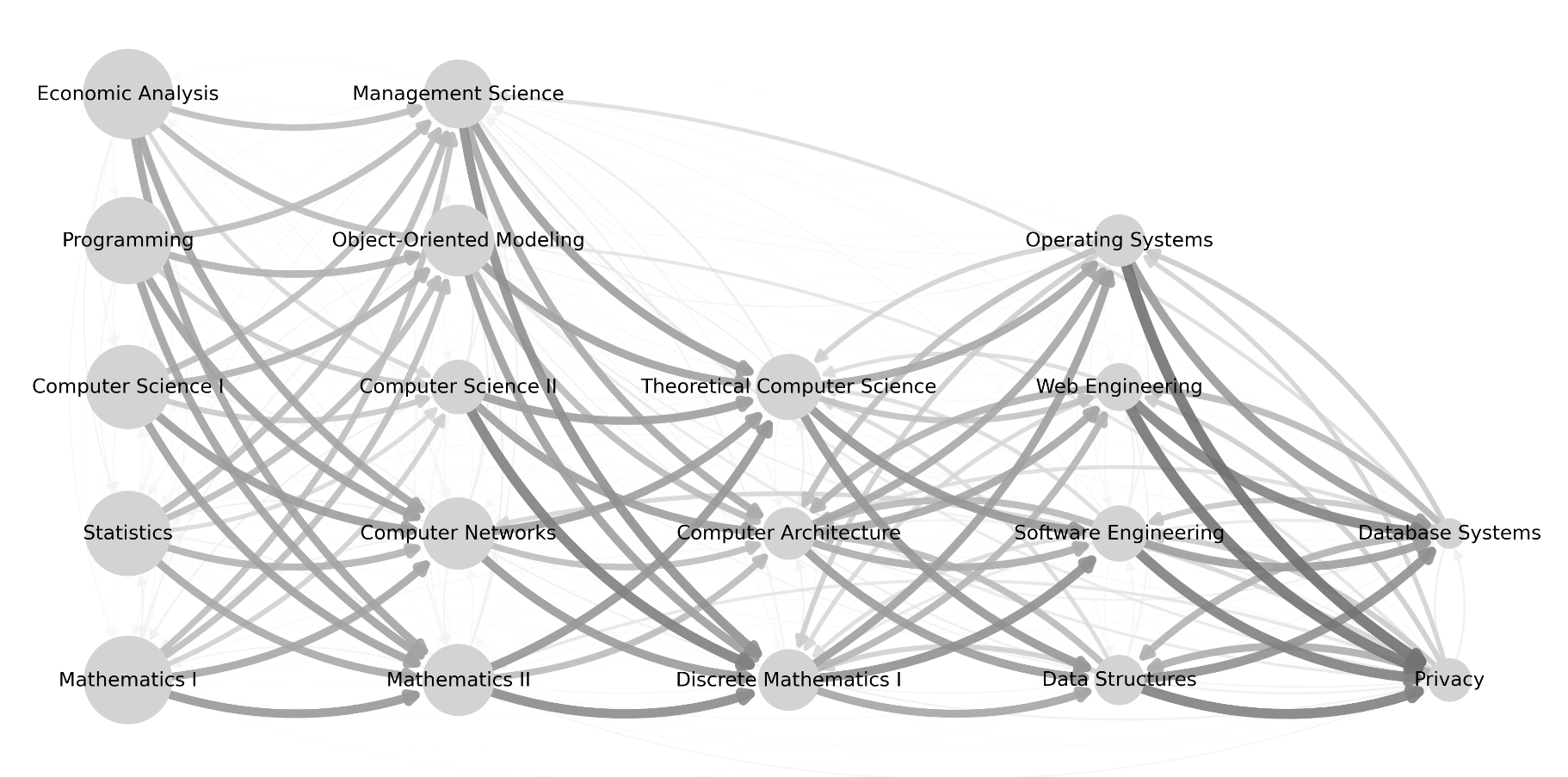
A student is usually located on several vertices at the same time within one semester depending on the number of courses he/she is attending. Figure 1, generated using NetworkX [10], shows the complexity of the flow. Here the courses are arranged as recommended by the curriculum. From left to right in semester ascending order the courses in one column belong to one semester. For example, the first column corresponds to the first semester. The course vertex size corresponds to the number of students that managed to finish the course. The graph is highly connected ( of possible edges) because in a lot of courses students violate the recommended curriculum. The darkness and thickness of edges indicate the weight of the flow. If an edge between two vertices corresponds to the weight value , it means that all students who attended course in one semester attended course in the next semester. The edges in Figure 1 suggest that the flow for the majority of students is from left to right according to the recommended curriculum. From the later semesters, when the amount of data decreases, the flow starts to become more chaotic, for example students move from right to left. This suggests that the observed students adhere less to the study plan as they progress in the degree program.
3.2 Degree Completion Time Simulation
The DCT-SIM consists of three steps: Initialization, course selection, and pass/fail prediction. The DCT-SIM of a student is completed, when all courses are passed. In one DCT-SIM run, we sample every student of group exactly once.
3.2.1 Initialization
We initialize each student of by having him/her attend a random subset of all the courses recommended for the first semester up to the workload that was extracted from the data of that specific student. If a student has a workload in the first semester, that exceeds the workload of all first semester courses, we assign second semester courses randomly until the workload is filled. We identified a statistically significant correlation between the grades of the courses in the first semester. We intended to include the correlation via a multivariate Gaussian distribution in the initialization. Unfortunately, the grade distributions of the courses are multi-modal. Therefore, we sample from the grade combinations of the first semester given by the data of the specific student that gets simulated. In that way, we can incorporate the grade correlations of the first semester courses as well.
3.2.2 Credit Workload and Course Selection
Various factors play a role when a student chooses the workload for an upcoming semester [12]. When simulating students from group , we draw the workload from the data of the specific student that gets simulated. If a workload of is drawn, it is randomly re-drawn from the normal distribution with the mean and the standard deviation of the workloads of other students from group in that semester. This happens, for example, when a student has not taken any courses in a semester. If the DCT-SIM leads to semesters in which no data are available, a workload of credits is set. Next, we need to select courses to fulfill the chosen workload. Courses are randomly drawn based on the student flow graph as follows. First, the courses that have not been passed before are selected. Given the remaining workload, we draw courses based on the courses already passed using the graph until the workload is reached. For this purpose, we go through the passed courses in random order. For each passed course, we draw one course from the not yet passed neighboring courses from , which are connected to the current course via edges from . The associated transition rates are used in the drawing process as transition probabilities. If a course is selected, it can no longer be drawn over other courses.
3.2.3 Pass/Fail Prediction
Grade prediction depends on the quality of the data that is available. Group consists of students who have very low failure rates, as we have shown above. To examine which is a good prediction method for all data in our data set, we want to obtain a subset that is as representative as possible. We consider student groups , which contain all students who attempted all courses from term . This gives us the cardinalities , , , , and . To test the accuracy of different methods, we calculate the average accuracy values over all terms . In addition, we limit ourselves to the labels "passed" and "failed". As a baseline, we use the prediction that always predicts the most frequent class ’passed’ () and compare it with the following methods. The first method ’Global’ draws ’pass’ with the average pass rate as probability, independently of course and student. The method ’Course’ uses course-specific pass rates and the method ’Student’ uses student-specific pass rates. In addition to these simplified methods, we use Naive Bayes and Decision Tree, implemented using scikit-learn [16], based on the promising results in past studies [2]. Balanced accuracy (bACC) defined as
is used as a measure of accuracy, where TP/FP and TN/FN are the true/false positives and true/false negatives, respectively [6]. In addition to predicting new grades, grades must also be predicted when a student repeats a course exam. We have seen that repeating students perform better on average in the second attempt of an exam. If a student fails an exam, the grade of the next try is predicted to be the old grade plus a grade bonus, which equals the average performance gain of . To fit the grade scale, the grade bonus is rounded up to . It is further assumed that the bonus applied from the second to the third attempt does not differ from the bonus applied from the first to the second attempt.
3.2.4 DCT Simulation Assumptions
The following summarizes the assumptions used for the DCT-SIM.
- All courses can be attended every semester and all students attend courses every semester.
- Workload and first semester grades are drawn from the data.
- If a student’s drawn workload is , we draw a workload from the normal distribution given the mean and the standard deviation of the other student’s workloads.
- If we need to draw workloads without a data basis, we set them to .
- Students do equally better in all courses when they retake an exam (grade bonus ).
- DCT-SIM finishes when every course is finished.
3.3 Policy Changes
Policy changes to the curriculum are a powerful tool to change student behavior. Its use should be all the more careful. Our DCT-SIM offers the ability of an approximate evaluation of these sensitive changes. First, we consider the workload. Since the proposed number of courses in the first semester results in a workload of credits, we examine the effect of changing the workload. We simulate the impact of increasing the workload by exactly one course, which corresponds to a minimum of credits. Second, we consider the course exams. In the current curriculum, one exam per semester is offered. This is different in other degree programs where there are two exams every two semesters or even two exams every semester. This means that students may be able to continue their studies without delay even if they do not pass the first exam. The policy changes are summarized as follows:
- ’Workload’: credit raise of workload in the first term,
- ’Exam (2-2-2)’: Every exam takes place twice every term,
- ’Exam (2-0-2)’: Every exam takes place twice only every two terms.
3.4 Evaluation Metrics
As in Fiallos et al. [9], we use the mean DCT to compare two DCT distributions to benchmark our results. The authors additionally used a Mann-Whitney U test to evaluate the statistical significance of the simulated DCT distribution. The test can support the alternative hypothesis that two samples correspond to different probability distributions rejecting the null hypothesis that the corresponding distributions are equal. Since the -value is defined as the conditioned probability of the observed statistic conditioned on the null hypothesis, a high -value fails to reject the null hypothesis but does not necessarily accept it [24]. Therefore, we will instead simulate individuals and thus introduce a DCT based error measure using the ground truth DCT as
where corresponds to the number of DCT-SIM runs. In the following, we set .
4. RESULTS
| Score \Methods | Baseline | Global | Course | Student | NB | DT |
|---|---|---|---|---|---|---|
| TP | ||||||
| FP | ||||||
| TN | ||||||
| FN | ||||||
| bACC |
4.1 Pass/Fail Prediction and DCT Simulation
Since in the baseline method we always assume label ’pass’, the true positives (TP) correspond to the actual pass rate and the false positives (FP) to the actual failure rate across all courses in the degree program. Table 4 shows the pass/fail prediction results of the various methods. For the baseline method the true positive percentage (TP) is high reflecting that the pass rate across all courses in the degree program is . The balanced accuracy (bACC) is . We note that the accuracies of the Global () and Course () methods are not significantly greater than the baseline. On the other hand, the Student method () achieved the best values for true negative and false negative percentages. The Naive Bayes method achieved the highest true positive percentage, while the Decision Tree method had the best overall bACC with and the best false positive percentage. Therefore, we used the Decision Tree method in the DCT-SIM.
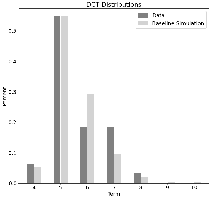
Figure 2 shows the DCT distributions of the DCT-SIM in light grey and the data in dark grey. The bars indicate the average percentage values achieved over a total of simulation runs. The DCT distributions of the simulation and the data reveal similar values in terms and . In the other terms, when the data of the group are sparser, since most of the students already completed all courses, the accuracy of the DCT-SIM also decreases noticeably. However, there is a small error of between the mean values of the DCT distributions with a p-value of , which is comparable to Fiallos et al. [9]. According to our DCT based error measure, we reach a value of This value corresponds to an average individual DCT error of semesters.
4.2 Policy Changes
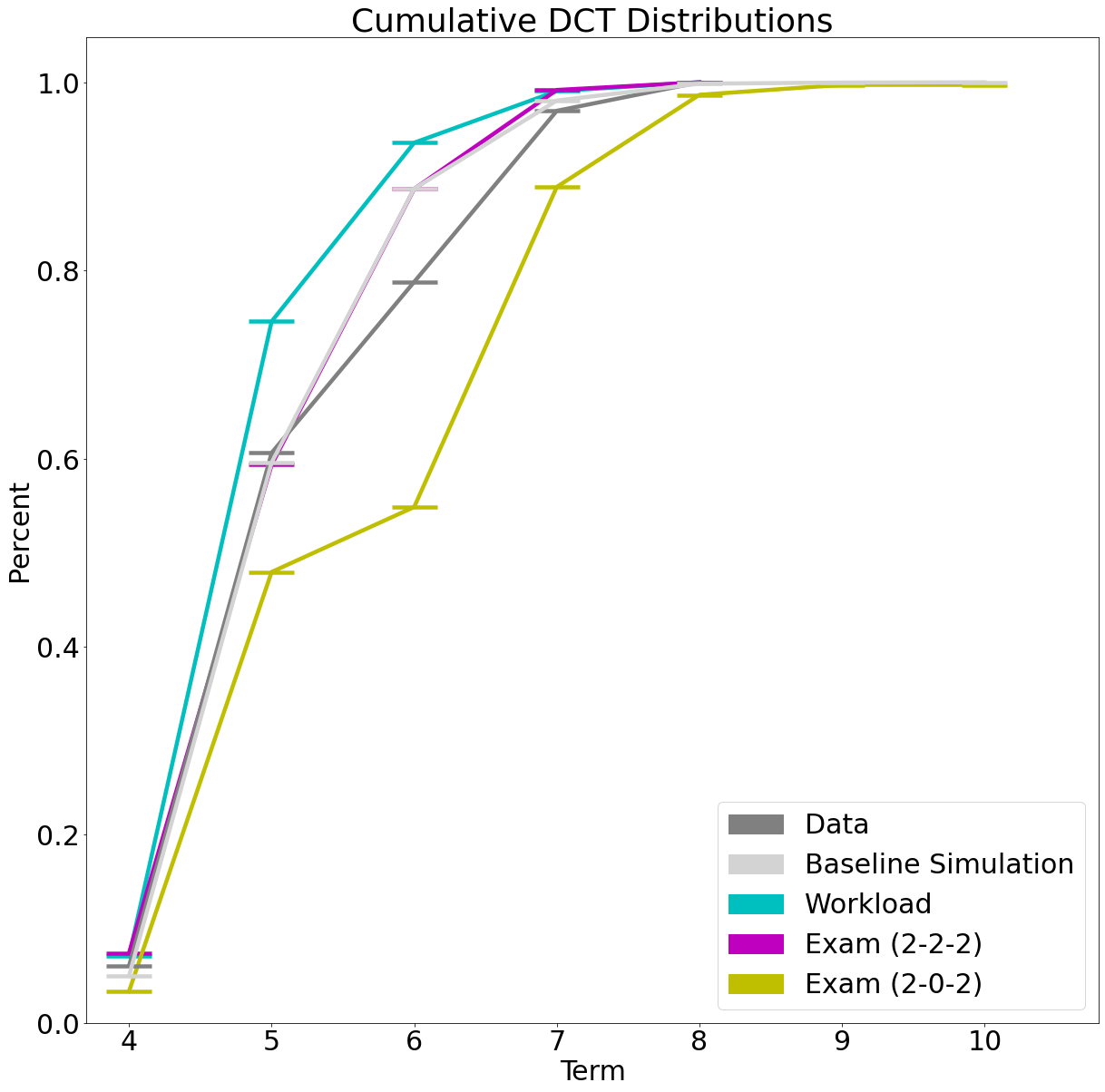
In the DCT simulations of the policy changes, for the sake of clarity, we have chosen a cumulative representation of the DCT distributions in Figure 3. The two graphs in gray correspond to the distributions of the data and baseline DCT-SIM as shown in Figure 2. We see that the workload change appears to be very effective, as the graph appears to be consistently above that of the baseline DCT-SIM. It turns out to be an improvement in the DCT means of . Thus, this change leads to a shortening of the DCT. The minor improvement of by policy change ’Exam (2-2-2)’ is only noticeable from term . In contrast, the policy change ’Exam (2-0-2)’ leads to a global increase of the DCT of .
5. DISCUSSION AND LIMITATIONS
We were able to show that student-dependent pass/fail prediction using the groups performs better than the assumption of a global pass rate or a course-specific pass rate. Overall, it is worthwhile to use the existing student performance data to increase accuracy.
Regarding the DCT-SIM, research in student flow simulation lacks good evaluation methods. Evaluation methods on the individual student level are missing, instead global DCT or dropout distributions are compared with the ground truth. This is due to the lack of use of labeled data and the resulting loss of assignability of students to their simulated counterparts. Using our generalizing approach, we were able to obtain comparable mean DCT errors on a global scale. In addition, through the intensive use of data, we were able to evaluate our DCT-SIM individually for each student from group . The error measure has shown that the evaluation with an average individual misfit of can be quite high without having a globally large effect. This results in the necessity to specify the goodness of fit of a DCT-SIM not only on a global level in the form of a mean DCT. We believe that a good DCT-SIM should be able to simulate each student as accurately as possible. Otherwise, a practical implementation of changes based on the observed DCT-SIM could lead to unexpected dynamics and thus to unfair conditions for an individual student. Policy changes for a curriculum are a relevant use case for a DCT-SIM because a data-generating process is needed to produce results. For our approach, we could identify two types of changes: Additive policy changes and restrictive policy changes. The former is characterized by changes in the frequency or acceleration in time of exams. For example, an increase in workload conditions the speed at which courses can be attended. The latter type, under which the ’Exam (2-0-2)’ change falls, directly restricts the frequency of exams in every second term. Our method was able to evaluate changes in the first category very well. The policy changes ’Workload’ and ’Exam (2-2-2)’ show plausible results. In particular, ’Exam (2-2-2)’ equates to a global increase in pass rates in our setting, due to the assumption of a grade bonus when repeating an exam. Since we have shown that students from group have very high pass rates, it makes sense that the effect is small for this group.
The ’Exam (2-0-2)’ change appears to be leading to a global extension of DCT. We have seen that the policy change ’Exam (2-2-2)’ behaves similarly to the baseline simulation. Therefore, we conclude that the policy change ’Exam (2-0-2)’ also behaves similarly to the policy change ’Exam (1-0-1)’. We point out the step-shaped graph in Figure 3. Looking at the number of courses per semester in Figure 1 and the average semester workloads of group in Table 3, we see that in semesters , and the average workload difference from the recommended workload is higher than in semesters and . Thus, the case occurs where a student has completed all subjects from semesters and in semester , but is missing subjects from semesters , and that cannot be completed until semester or even . As a result, few students finish in or semesters, as seen in Figure 3. This shows the still existing rigidity of our workload approach. We believe that predicting workload as a function of courses, grades, and exam attempts, rather than deriving it directly from the student being simulated, may lead to a more robust DCT-SIM with respect to policy changes.
Awareness regarding algorithmic bias and fairness is emerging in the field of Educational Data Mining. Especially when a model gets implemented in practice so that students are affected in their learning environment, an identification of bias and fairness of the data and methods used as well as their resulting actions have to be assured [4, 11]. In addition to the mentioned limitations of our method, we are aware of the performance bias (i.e. we mainly consider successful students) in the data used and would like to remove it in the future by expanding and balancing our data set.
In terms of computational power, we observe a time consumption for one non parallelized DCT-SIM of student group : , using an Intel(R) Core(TM) i5-6200U CPU @ 2.3GHz processor.
With respect to the DCT mean, we were able to obtain a comparatively well-fitting DCT distribution from our DCT-SIM in which only student data were processed. The dependence on the data offered us the ability to construct a student flow based curriculum graph in a maximally flexible study plan, perform an individual evaluation of the DCT-SIM using the error measure and investigate and evaluate policy changes in a highly flexible curriculum. In this sense, we were able to generalize existing approaches. In order to implement our approach for university practitioners in the future, we will conduct further research. The first priority is the extension of the data set as well as achieving high individual accuracy. An ethical analysis with the involvement of student and teacher representatives is planned.
6. ACKNOWLEDGMENTS
We thank Agathe Merceron for her valueable feedback. The work is supported by the Ministry of Culture and Science of the state of NRW, Germany through the project KI.edu:NRW.
7. REFERENCES
- P. R. Aldrich. The curriculum prerequisite network: Modeling the curriculum as a complex system. Biochemistry and Molecular Biology Education, 43(3):168–180, 2015.
- R. Asif, A. Merceron, S. A. Ali, and N. G. Haider. Analyzing undergraduate students’ performance using educational data mining. Computers & Education, 113:177–194, 2017.
- M. Backenköhler, F. Scherzinger, A. Singla, and V. Wolf. Data-driven approach towards a personalized curriculum. In 11th International Conference on Educational Data Mining, pages 246–251, 2018.
- R. S. Baker and A. Hawn. Algorithmic bias in education. International Journal of Artificial Intelligence in Education, pages 1–41, 2021.
- J. Banks. Handbook of simulation: principles, methodology, advances, applications, and practice. John Wiley & Sons, 1998.
- M. Bekkar, H. K. Djemaa, and T. A. Alitouche. Evaluation measures for models assessment over imbalanced data sets. Journal of Information Engineering and Applications, 3:27–38, 2013.
- A. Bogarín, R. Cerezo, and C. Romero. A survey on educational process mining. Wiley Interdisciplinary Reviews: Data Mining and Knowledge Discovery, 8(1):e1230, 2018.
- E. Caro, C. González, and J. M. Mira. Student academic performance stochastic simulator based on the monte carlo method. Computers & Education, 76:42–54, 2014.
- A. Fiallos and X. Ochoa. Discrete event simulation for student flow in academic study periods. In 2017 Twelfth Latin American Conference on Learning Technologies (LACLO), pages 1–7. IEEE, 2017.
- A. Hagberg, P. Swart, and D. S Chult. Exploring network structure, dynamics, and function using networkx. Technical report, Los Alamos National Lab.(LANL), Los Alamos, NM (United States), 2008.
- R. F. Kizilcec and H. Lee. Algorithmic fairness in education. arXiv preprint arXiv:2007.05443, 2020.
- E. Kyndt, I. Berghmans, F. Dochy, and L. Bulckens. ’time is not enough.’workload in higher education: a student perspective. Higher Education Research & Development, 33(4):684–698, 2014.
- S. Mansmann and M. H. Scholl. Decision support system for managing educational capacity utilization. IEEE Transactions on Education, 50(2):143–150, 2007.
- R. Molontay, N. Horváth, J. Bergmann, D. Szekrényes, and M. Szabó. Characterizing curriculum prerequisite networks by a student flow approach. IEEE Transactions on Learning Technologies, 13(3):491–501, 2020.
- M. Pechenizkiy, N. Trcka, P. De Bra, and P. Toledo. Currim : Curriculum mining. In Proceedings of the 5th International Conference on Educational Data Mining, EDM 2012, pages 216–217. International Educational Data Mining Society (IEDMS), 2012.
- F. Pedregosa, G. Varoquaux, A. Gramfort, V. Michel, B. Thirion, O. Grisel, M. Blondel, P. Prettenhofer, R. Weiss, V. Dubourg, J. Vanderplas, A. Passos, D. Cournapeau, M. Brucher, M. Perrot, and E. Duchesnay. Scikit-learn: Machine learning in Python. Journal of Machine Learning Research, 12:2825–2830, 2011.
- M. Raji, J. Duggan, B. DeCotes, J. Huang, and B. V. Zanden. Modeling and visualizing student flow. IEEE Transactions on Big Data, 7(3):510–523, 2021.
- C. Romero and S. Ventura. Educational data mining and learning analytics: An updated survey. Wiley Interdisciplinary Reviews: Data Mining and Knowledge Discovery, 10(3):e1355, 2020.
- R. M. Saltzman and T. M. Roeder. Simulating student flow through a college of business for policy and structural change analysis. Journal of the Operational Research Society, 63(4):511–523, 2012.
- A. Schellekens, F. Paas, A. Verbraeck, and J. J. van Merriënboer. Designing a flexible approach for higher professional education by means of simulation modelling. Journal of the Operational Research Society, 61(2):202–210, 2010.
- A. Slim, G. L. Heileman, J. Kozlick, and C. T. Abdallah. Employing markov networks on curriculum graphs to predict student performance. In 2014 13th International Conference on Machine Learning and Applications, pages 415–418. IEEE, 2014.
- A. Slim, G. L. Heileman, J. Kozlick, and C. T. Abdallah. Predicting student success based on prior performance. In 2014 IEEE symposium on computational intelligence and data mining (CIDM), pages 410–415. IEEE, 2014.
- P. Voigt and A. Von dem Bussche. The eu general data protection regulation (gdpr). A Practical Guide, 1st Ed., Cham: Springer International Publishing, 10(3152676):10–5555, 2017.
- R. L. Wasserstein and N. A. Lazar. The asa statement on p-values: context, process, and purpose, 2016.
- J. Wigdahl, G. L. Heileman, A. Slim, and C. T. Abdallah. Curricular efficiency: What role does it play in student success? In 2014 ASEE Annual Conference & Exposition. ASEE Conferences, 2014.
© 2022 Copyright is held by the author(s). This work is distributed under the Creative Commons Attribution-NonCommercial-NoDerivatives 4.0 International (CC BY-NC-ND 4.0) license.