ABSTRACT
Many models of categorization focus on how people form and use knowledge of categories and make predictions about human categorization behaviors [19]. However, few (if any) of them implement these theories into item selection algorithms for category training. The performance Factors Analysis (PFA) model is an alternative to the Bayesian Knowledge Tracing model that tracks students’ learning of knowledge components and can be implemented into adaptive practice algorithms [17]. PFA-Difficulty model has been built to select items based on their difficulty level adaptively [4]. This paper describes how we are working to incorporate categorization theories into the PFA model so that it can be used for item selection. We used experiment data of Mandarin tone categorization training to test the model and suggest the implications of the results for item selection.
Keywords
INTRODUCTION
Formal models of categorization make assumptions about human psychological processes during categorization [8,19]. They specify three things in general: (1) the internal representation of the content and format of categorical knowledge, (2) the retrieval process that collects the exact information needed to make a response, (3) the response selection process about how to select a response based on the information collected [2,13]. However, categorization models do not consider individual differences in learning categories and do not track learners’ learning process. Therefore, they cannot help instructional design about item selection for training because most processes of learning (other than categorization) are not characterized in the models, e.g., the benefit of active quizzing.
For example, exemplar theory assumes that subjects store each distinct stimulus and its category label in prior memory. To classify a stimulus, subjects compute the similarities between the stimulus representation and all the stored representations of exemplars, aggregate the similarities, and then make a categorical selection [13,19]. But such a strict exemplar theory is not accurate based on what we know about how the brain encodes memories [3]. Analogously, a prototype model operates by computing the similarities between the instances and a summary representation in memory. The difference is that the prototype model assumes that subjects store a “prototype”, which could be a central tendency of that category instead of every exemplar [13,19]. Importantly, neither of the above models care about training sequence. More recently, Sequential Attention Theory Model (SAT-M) was developed using local context, which considers the influence of the properties of temporally neighboring items during training [5]. However, the model is built based on the Generalized Context Model (GCM) [16], a special case of exemplar models, so it still implausibly supposes a person memorizes all prior instances. Even though it captures the influence of training sequence on the stimuli representation and improves the model fit for data with different training sequences, the model does not intend to give specific suggestions about item selection. The goal of this study is to implement the categorization theories into a learner model so that it can track learners’ learning of categories and provide suggestions on item selections for future training.
The Performance Factors Analysis (PFA) model is a student model that predicts individual students on knowledge components (KCs) [1] which are acquired units of cognitive function or structure (e.g., concept, fact, or skill) using counts of successes and failures on prior training trials [17,18]. The PFA model could help us develop adaptive training algorithms. Below are the formulas of the original Performance Factors Analysis model.
(1) |
(2) |
In Equation 1, i represents a student and j represents a KC. m is a logit value representing the accumulated learning of the students on KCs. βj represents the easiness of the specific KC. s and f count the sum of cases/trials of prior successes and failures. γ and ρ are parameters scaling the effect of the observation counts. In Equation 2, the accumulated learning is converted to probability prediction.
Even though, from the results of the PFA model, we can know whether correct or incorrect responses lead to more learning gains on each KC, the result can’t be used for item selection. The reason is that if the success coefficient γ is higher than the failure coefficient ρ, it implies us to select easier items that could achieve immediate success and then maximize the learning gains (the increase of m value) [4]. However, this is in opposition to some pedagogical theories, which suggest that medium-range difficulty of items promotes better learning. For example, the Goldilocks principle in cognitive science [11] and the zone of proximal development [21] suggest that the practices should be neither too simple nor too complex relative to learners’ current knowledge. Kelley [12] also stated that keeping an appropriate difficulty level can make training effective. If a task is too easy, it will result in low levels of mental effort, whereas if the task is too difficult, it will be difficult to encode the experience. Both cases lead to low learning gains. Therefore, we hypothesized that the relationship between difficulty and learning gains could be expressed as an inverted-U function (see equation 3) and incorporate it into the PFA model to build a new model called PFA-Difficulty (see equation 4) [4].
(3) |
In equation 3, x represents the difficulty of the item. y represents the effect of difficulty on learning gains. In Equation 4. instead of tracking counts of prior successes and failures, we track the effects of prior difficulty levels of successes and failures using quadratic equations.
(4) |
We have tried to use the PFA-Difficulty model to select the item with optimal difficulty level for practice. However, the model is not the most appropriate model for categorization. It does not involve learners’ categorization process like the prototype and exemplar models do. Furthermore, even though we can treat categories as knowledge components and find the optimal difficulty to learn for each category, there is no suggestion about how to select items between categories. Therefore, this study intended to build a PFA model variant that implements a categorization theory while remaining simple enough to implement for adaptive practice.
METHOD
Dataset
We used a dataset from a Mandarin tone training experiment [4] as a test case for the new model. Two hundred and five participants (Female = 89, Male =116) who were Amazon Mechanical Turk workers reside in Canada or the US. Age ranged across the lifespan: 10.2% were between 18-25 years old, 34.6% were 26-34, 45.4% were 35-54, and 7.8% were 55-64 years old. Only 2.0% were more than 65 years old. The survey question for education level showed that 12.7% had a high school diploma or GED, 42.0% had some college, 38.5% had a 4-year college degree or bachelor’s, and 6.8% had a graduate degree. They finished 216 trials of training in Mandarin tones in the experiment. There are four Mandarin tones (Tone 1, a high-level tone; Tone 2, a rising tone; Tone 3, a low falling-rising tone, and Tone 4, a falling tone). In each trial, participants listened to a tone sound and selected from the four options which tone it was.
Stimulus representation
The representation of stimuli could be derived from multidimensional scaling (MDS), additive clustering, and factor analysis. Based on the results of previous MDS studies of Mandarin tones [7,10] and the experiment design, we encoded the tone stimuli in 7 features. Three of them are about the F0 (fundamental frequency) direction (level, rising, and down). The other four are about the experiment variables (duration, expansion, and speaker gender).
PFA-Categorization
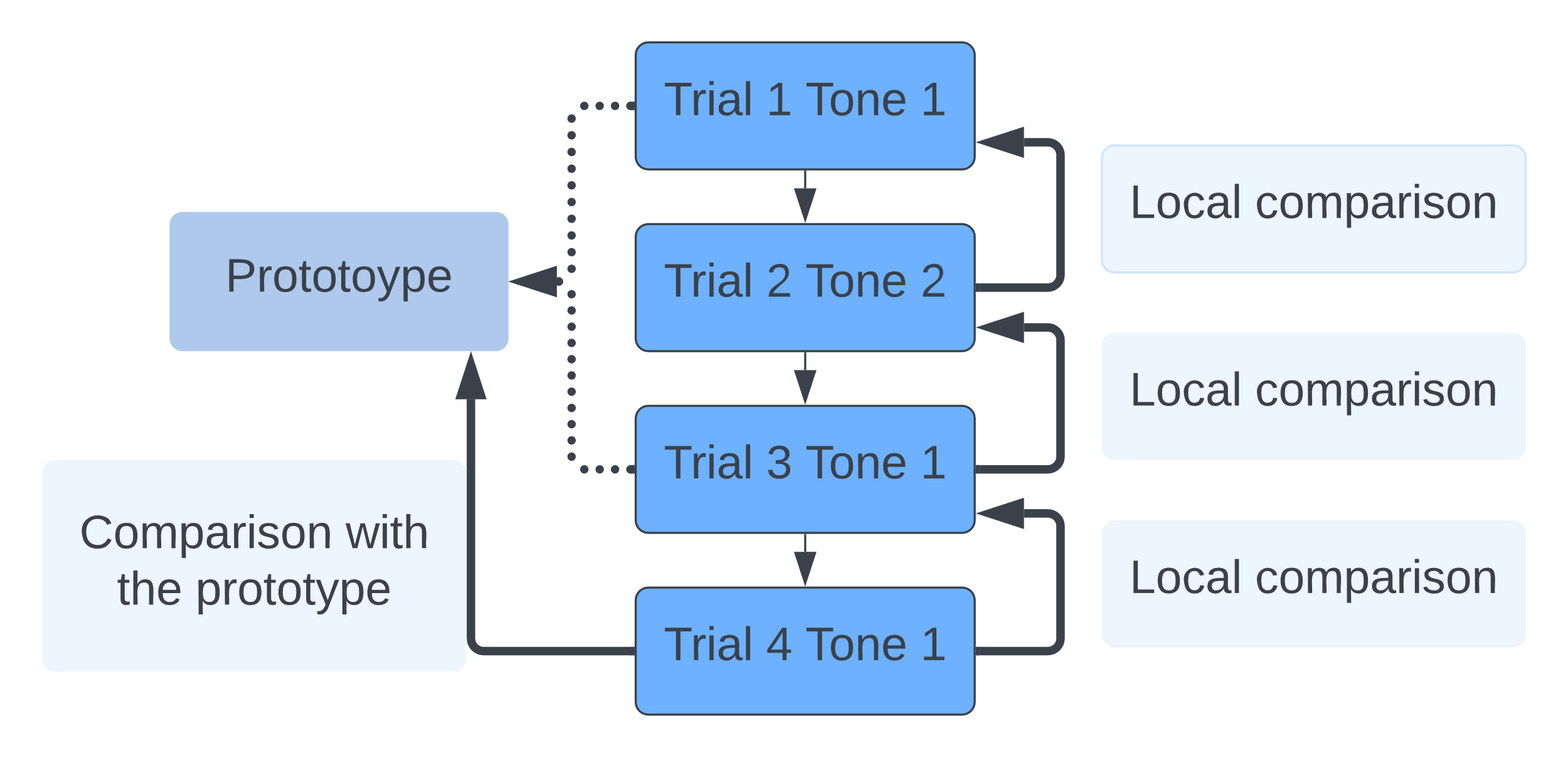
Based on exemplar and prototype theories, learners learn through comparing the similarity between the new instance with previous exemplars and prototypes. Here for simplification, we used a prototype mechanism where learners compare the new instance with the prototype of that category. The prototype is calculated by the average feature values of previous examples of the belonging category. According to the SAT-M model, local context is also important. Learners should also learn from comparing the similarity between the new instance and its previous neighboring item. Therefore, the model should track two types of comparisons: the comparisons with the prototype and the local prior trial.
For the relationship between learning gains and similarity, we have a similar hypothesis to the relationship between learning gains and the difficulty level, which can also be expressed using the simple quadratic function. If the two compared objects are too similar, it will be either too difficult if they belong to different categories or too easy if they are from the same category, and vice versa. Therefore, the medium-range similarity might be optimal for practice. Then the equation of the new PFA-Categorization model can be shown as follows (see equation 5).
(5) |
L represents the local comparisons between the current trial and its previous trial by calculating the similarities between the two items for each KC). P indicates the comparisons to the prototype by calculating the similarities between the current trial and its prototype for each KC). γ1 and γ2 are scaling the effects of local comparisons of prior successes. ρ1 and ρ2 are parameters scaling the effects of local comparisons of prior failures. Similarly, γ3 and γ4 and ρ3 and ρ4 are parameters scaling the comparisons with prototypes. In this study, for simplification, we used the Euclidean distance as an index of similarity between two items (see equation 6). Parameters p and q represent the to be compared two objects. r is the dimension of the features that range from 1 to n. pr and qr are the feature values of objects p and q on dimension r.
(6) |
Statistical Analysis
The knowledge components in the Mandarin tone training data are four Mandarin tones. Figure 1 shows an example of the local comparisons and the prototypes’ comparisons using four trials of experiment data. The bold solid arrows represent the comparisons, and the dashed arrow indicates the formation of the prototype. The thin solid arrows show the direction of the training sequence. We used the category of previous trials as covariates for the local comparisons when tracking the similarities between the current trial and the previous neighboring trial. The prototype is calculated by averaging the features of previous learned examples of that category. We then used the new PFA-Categorization model to analyze the data and computed the logit function increase or decrease as a function of similarity on each tone. All analyses were completed in R, with source code available from the corresponding author.
RESULTS
We did 5-fold cross-validations for the PFA, PFA-Difficulty, and PFA-Categorization models and calculated the mean test fold R2 (see Table 1). An R package “LKT” (Logistic Knowledge Tracing) [18] was used to do the analysis. In all the models, we used the stimuli (Problem.Name) as the intercept. Tone represents the knowledge components (KCs) in the dataset. In the PFA model, linesuc$ and linefail$ track the counts of prior successes and failures of each KC. While in the PFA-Difficulty model, diffcor1$ and diffcor2$ are used to track the effects of difficulty levels of prior successes, and diffincor1$ and diffincor2$ are used to track the effects of difficulty levels of prior failures. Similarly, in the PFA-Categorization model, we used those parameters to track the effects of local similarities and similarities to the prototype. From the R2 values of the three models, there are minor differences among them, which means they fit the data equally well.
The local comparisons are more closely related to the training sequence than the prototype comparisons. Since the training sequence of the experiment was in random order, there are 16 pairs of local comparisons (4 tones * 4 tones). We used the coefficients of the local comparisons in the PFA-Categorization model to compute the learning efficiency (learning gains divided by the time cost) [9] as a function of the distance levels. The learning gain means the increase or decrease of the m value in equation 5. Table 2 shows an example of the learning gains calculation when Tone 1 is the previous trial and Tone 1, Tone 2, Tone 3, or Tone 4 is the current trial. The distance value was normalized to be in a range of 0 and 1, which was initially between 0 and 5.76.
Local comparisons | The function logit change |
|---|---|
Tone 1-Tone 1 | x*(0.30*x-0.30*(x)2) + (1-x) *(-0.33*x+0.30*(x)2) |
Tone 1-Tone 2 | x*(-0.12*x+0.20*(x)2) + (1-x) *(-.03*x+0.12*(x)2) |
Tone 1-Tone 3 | x*(0.19*x-0.08*(x)2) + (1-x) *(-0.17*x+0.18*(x)2) |
Tone 1-Tone 4 | x*(0.21*x+0.00*(x)2) + (1-x) *(-0.29*x+0.22*(x)2) |
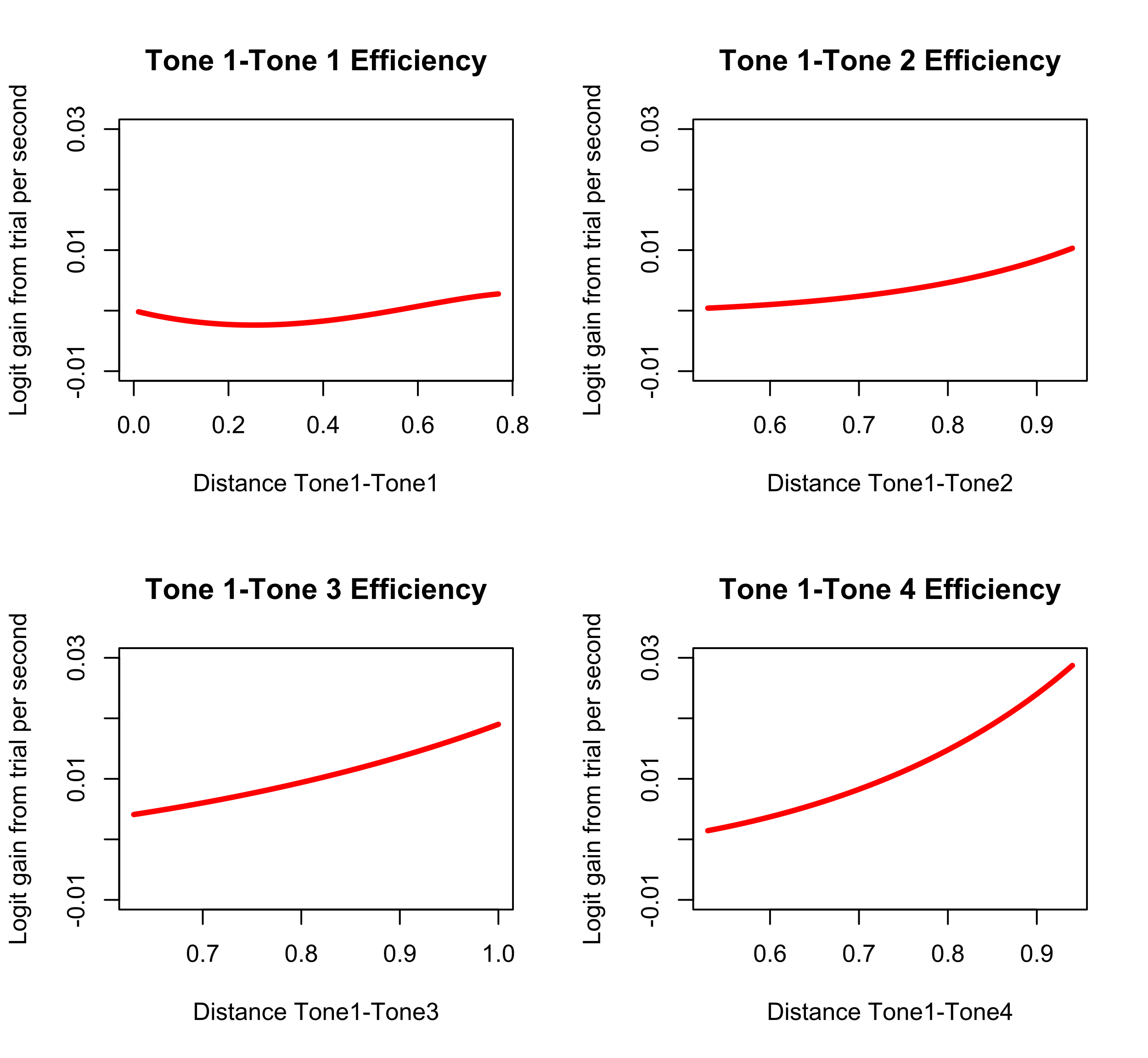
Then we plotted the learning efficiency of the local comparison pairs and found the maximum values of logit change per second given the distance between two tones. For example, Figure 2 shows the learning efficiency curves of local comparisons when Tone 1 is the previous tone, and the adjacent current tone could be Tone 1, Tone 2, Tone 3, or Tone 4. For the Tone 1-Tone 1 pair, the logit gain from trial per second is the largest when the distance between them is 0.83, and the maximal learning gain per second is 0.003. For Tone 1-Tone 2 pair, Tone 1-Tone 3, and Tone 1-Tone 4, the optimal distance values are 1, 1, and 1, and the maximal learning gain is 0.014, 0.019, 0.037, respectively. Therefore, to achieve the maximal learning gain when practicing Tone 1, we should select Tone 4 as the next learned item. Similarly, after analyzing Tone 2, Tone 3, and Tone 4 as the previous trial separately, the findings suggest that we select Tone 4, Tone 1, and Tone 3, respectively, to achieve maximal learning gain. Above findings are just the first step to build an adaptive training system since we only have a static prediction about which tone category to select. The predictions are not sensitive to learners’ performance changes due to learning. Adaptive training not only needs to consider individual differences (learning rate) but also needs to adjust the similarity between practice trials accordingly to achieve the maximal learning gain for individuals. That is the direction for future work which is out of the scope of this preliminary report.
DISCUSSION
In this study, we are combining categorization theories with the PFA model to track learners’ learning of categories. Instead of tracking counts of prior successes and failures as the PFA model does or effects of difficulty levels of prior successes and failures as the PFA-Difficulty model does, the new PFA-Categorization model tracks the similarities between the adjacent trials and the similarity between each trial and its prototype of the belonging category. The R2 values showed that the performance of the PFA-Categorization model was better than the original PFA model. Even though the quantitative comparison did not reveal differences, it has useful implications for later item selection for category training. After learning a specific tone category, it may be possible to make decisions about what category and item are to be practiced next.
Many studies have examined the influence of presentation order of examples on category learning [6,14,20]. For example, Carvalho and Goldstone [6] suggest that if stimuli have high within- and between-category similarity interleaved study could result in better generalization, whereas if categories have low within- and between-category similarity, blocked presentation can lead to better generalization. However, their study used extreme examples of similarities that are either too similar or too dissimilar, which is not so often seen in regular category learning. They also have no systematic suggestion about how we should sequence the categories based on their similarity levels and learning gains. Prior studies have simple manipulations about similarity either maximize or minimize the similarity between adjacent training trials [14,15]. These methods are too general and may not fit all the category learning cases. The benefit of the PFA-Categorization model is that it could give us suggestions about what we should select next based on the analysis of the training data to achieve maximal learning efficiency.
CONCLUSION
This paper implemented a categorization mechanism into the PFA model to track category learning that suggests what category we should select next based on the learning efficiency curve as a function of the similarity between the two adjacent items. We plan to use a developed version of the model in an adaptive training system to select the item with optimal similarity levels for learners to achieve maximal learning efficiency.
Future work will improve the model by adding weights of features into the distance calculation since different features may have different importance for categorization. We will also test the model with more datasets since the data used in the present study did not have any manipulation of practice schedules so it may not work well for the data. For example, interleaved practice and blocked practice may have different types of local comparisons that the former is mainly between-category comparisons, and the latter is within-category comparisons. However, since the practice data we used mixed between and within category comparisons randomly it is difficult to see the cumulative effects of scheduling strategy in the data.
REFERENCES
- Aleven, V., & Koedinger, K. R. 2013. Knowledge component (KC) approaches to learner modeling. Design Recommendations for Intelligent Tutoring Systems, 1, 165-182.
- Ashby, F. G., & Maddox, W. T. 1993. Relations between prototype, exemplar, and decision bound models of categorization. Journal of Mathematical Psychology, 37(3), 372-400.
- Bowman, C. R., Iwashita, T., & Zeithamova, D. (2020). Tracking prototype and exemplar representations in the brain across learning. Elife, 9, e59360.
- Cao, M., Pavlik Jr, P. I., & Bidelman, G. M. 2019. Incorporating Prior Practice Difficulty into Performance Factor Analysis to Model Mandarin Tone Learning. In Lynch, C. F., Merceron, A., Desmarais, M., & Nkambou, R. (Eds.), Proceedings of the 12th International Conference on Educational Data Mining (pp. 516 - 519). Montreal, Canada.
- Carvalho, P. F. & Goldstone, R. 2019. A computational model of context-dependent encodings during category learning. PsyArxiv. https://doi.org/10.31234/osf.io/8psa4.
- Carvalho, P.F. and Goldstone, R.L. 2014. Putting category learning in order: Category structure and temporal arrangement affect the benefit of interleaved over blocked study. Memory & Cognition. 42, 3 (Apr. 2014), 481–495. DOI:https://doi.org/10.3758/s13421-013-0371-0.
- Chandrasekaran, B., Sampath, P. D., & Wong, P. C. 2010. Individual variability in cue-weighting and lexical tone learning. The Journal of the Acoustical Society of America, 128(1), 456-465.
- Chandrasekaran, B., Koslov, S.R. and Maddox, W.T. 2014. Toward a dual-learning systems model of speech category learning. Frontiers in Psychology. 5, 825. DOI:https://doi.org/10.3389/fpsyg.2014.00825.
- Eglington, L. G., & Pavlik Jr, P. I. 2020. Optimizing practice scheduling requires quantitative tracking of individual item performance. NPJ science of learning, 5(1), 1-10.
- Gandour, J. T. 1978. Perceived dimensions of 13 tones: a multidimensional scaling investigation. Phonetica, 35(3), 169-179.
- Halpern, D.F., Graesser, A. and Hakel, M., 2008. Learning principles to guide pedagogy and the design of learning environments. Washington, DC: Association of Psychological Science Taskforce on Lifelong Learning at Work and at Home.
- Kelley, C.R., 1969. What is adaptive training? Human Factors, 11(6), pp.547-556.
- Kruschke, J. K. 2008. Models of categorization. In R. Sun (Ed.), The Cambridge handbook of computational psychology (Cambridge Handbooks in Psychology, pp. 267-301). Cambridge:Cambridge University Press. https://doi.org/10.1017/CBO9780511816772.013.
- Mathy, F., & Feldman, J. 2009. A rule-based presentation order facilitates category learning. Psychonomic bulletin & review, 16(6), 1050-1057.
- Medin, D. L., & Bettger, J. G. 1994. Presentation order and recognition of categorically related examples. Psychonomic bulletin & review, 1(2), 250-254.
- Nosofsky, R. M. 1986. Attention, similarity, and the identification–categorization relationship. Journal of experimental psychology: General, 115(1), 39.
- Pavlik Jr, P. I., Cen, H., & Koedinger, K. R. 2009. Performance factors analysis -- A new alternative to knowledge tracing. In V. Dimitrova, R. Mizoguchi, B. d. Boulay, & A. Graesser (Eds.), Proceedings of the 14th International Conference on Artificial Intelligence in Education (pp. 531–538). Brighton, England.
- Pavlik, P. I., Eglington, L. G., & Harrell-Williams, L. M. (2021). Logistic Knowledge Tracing: A Constrained Framework for Learner Modeling. IEEE Transactions on Learning Technologies, 14(5), 624-639.
- Pothos, E. M., & Wills, A. J. (Eds.). 2011. Formal approaches in categorization. Cambridge University Press.
- Sandhofer, C. M., & Doumas, L. A. 2008. Order of presentation effects in learning color categories. Journal of Cognition and Development, 9(2), 194-221.
- Vygotsky, L., 1986. Thought and Language. MIT Press, Cambridge, Mass.
© 2022 Copyright is held by the author(s). This work is distributed under the Creative Commons Attribution-NonCommercial-NoDerivatives 4.0 International (CC BY-NC-ND 4.0) license.