ABSTRACT

In this study, we proposed an Online Item Response Theory Model (OIRT) by combining the Item Response Theory and Performance Factor Analysis (PFA) models. We fitted the proposed model with modified Variational Inference (VI) to perform real-time student and item parameter estimation using both simulated data and real time series data collected from an online adaptive learning environment. Results showed that modified VI parameter estimation method outperformed other Bayesian parameter estimation methods in efficiency and accuracy. We also demonstrated that OIRT tracked students’ ability growth dynamically and efficiently, it also predicted students' future performance with reasonable AUC given limited input features.

Keywords

INTRODUCTION

As time series data become increasingly prevalent in online learning system, tracking students' ability changes during their learning processes is important for the analysis of teaching and learning activity. There have been three commonly used models for estimating students' cognitive mastery: Item Response Theory (IRT) model is a general tool to provide a quantitative description of students' ability in academic testing. Knowledge Tracing (KT) model tries to predict a students' future performance through their historical interaction logs [5]. Performance Factor Analysis (PFA) [15] analyzes learning rates of students by considering multiple Knowledge Components (KCs) of each exercise item.

None of the above approaches are perfectly applicable to monitor students' ability changes in online learning. IRT roots on the assumption that students’ true abilities are fixed [18], which may not be true in online learning environment, because student abilities are dynamic. Bayesian KT only estimates binary hidden states (either mastery or non-mastery) and models each KC separately. Standard IRT and PFA models are not able to perform real-time parameter estimation due to model format or estimation methods.

In this study, we propose an Online Item Response Theory Model (OIRT) to track students' ability changes in real-time fashion using both simulation and real data.

In summary, the contribution of the work is three-fold: (1) propose OIRT model by estimating students' initial abilities, item difficulties as well as ability changes for different KCs; (2) modify Variational Inference (VI) [24] under OIRT model to track students’ ability changes; (3) compare the computational time and accuracy of the modified VI with other parameter estimation approaches, and demonstrate answer accuracy prediction by OIRT.

background

In this part, IRT and PFA models as well as common real-time parameter estimation approaches are briefly reviewed.

Item Response Theory Model

IRT is widely used in assessing student abilities and item difficulties due to its high interpretability. The one-parameter logistic (1PL) model [16] is given in Eq.1,

where $y_{\text{ij}}\$is the $i$-th student's response to the $j$-th item. $y_{\text{ij}} = 1$ indicates a correct answer and 0 otherwise. $\theta_{i}$ denotes the ability of the $i$-th student and $b_{j}$ denotes the difficulty of the $j$-th item. We developed our OIRT model based on 1PL model in Eq.1, but OIRT can be extended to 2 or 3PL IRT models [7,8] easily.

Performance Factor Analysis

IRT model only estimates a constant ability for each student and cannot model the changes of student abilities as learning proceeds [18]. To address this problem, especially in the adaptive online learning environment, Learning Factor Analysis (LFA) model [4] and PFA model [15] are proposed to further include the prior practice counts for each KC. Specifically, PFA model, an extension of LFA model, is given in Eq.2,

Here, $\beta_{k}$ is the difficulty of the $k$-th KC, $s_{i,k}$ and $f_{i,k}$ are the prior successes and failures of the $i$-th student on the $k$-th KC, $\gamma_{i,k}$ and $\rho_{i,k}$ are the learning rates of these observation counts, implying the effects of accumulated successes and failures ($s_{i,k}$ and $f_{i,k}$) on answer accuracy in the processes of learning.

Some other models also try to track the changes of student abilities in a short period [10, 13, 23]. The main principle here is to estimate the ability change, $\Delta\theta_{t}$, based on students' responses to items. We also follow this principle by modeling $\Delta\theta_{t}$ using learning rate parameters and their corresponding practice counts, which will be introduced in Section 3.

online item response model

Online Item Response Theory (OIRT) model is an extension of the existing PFA model. Suppose there are $N$ students, $M$ items covering a total of $K$ KCs, the OIRT model is given in Eq.3,

where $\theta_{i}$ and $b_{j}$ denote the $i$-th student's general ability and the $j$-th item's difficulty, respectively. Let $K$ be the total number of KCs covered by all the items, $\overset{⃑}{s_{i}}$ and $\overset{⃑}{f_{i}}$ are $K*1$ vectors containing successful and unsuccessful practice counts for the $i$-th student. $\overset{⃑}{\gamma_{i}^{s}}$ and $\overset{⃑}{\gamma_{i}^{f}}$ are the $K*1$ learning rate vectors for $\overset{⃑}{s_{i}}$ and $\overset{⃑}{f_{i}}$, respectively. $\overset{⃑}{T_{j}}$ is a pre-specified $K*1$ distributional vector of KCs for item $j$. The $\odot$ and $\bullet \$are element-wise product and dot product, respectively.

OIRT contains four extensions compared to PFA model in Eq.2. (1) An initial ability $\theta_{i}$ for each student is added in OIRT due to the prior knowledge of students. (2) Note that modeling item difficulty as $\sum_{k}^{}\beta_{k}$ in PFA is unreasonable in that the item with the same KCs will have same difficulty. To solve the problem, we added a unique difficulty $b$ for each item in OIRT. (3) Instead of using a binary vector indicating which item covers which KC, we used a distributional vector $\overset{⃑}{T_{j}}$ to avoid a bias (working on items with more KCs will lead to higher ability gain when adding up the learning effects of all KCs covered by an item) towards the items with many KCs. To construct $\overset{⃑}{T_{j}}$ , suppose we have a total of $K = 3$ KCs, if item $j$ covers KC 1 and 3, instead of representing the item-KC vector as $\lbrack 1,0,1\rbrack$, we represent it as$\overset{⃑}{\text{\ T}_{j}} = \lbrack 1/2,\ 0,\ 1/2\rbrack$, whose sum is always equal to 1. (4) The parameters in OIRT will be updated in a real-time mode: once a student receive the feedback after answering an item, we update $\overset{⃑}{s_{i}}$ and $\overset{⃑}{f_{i}}\$and hence the corresponding learning rate vectors, this is a major difference between OIRT model and other IRT and PFA models, because of the dynamic updates of $\ \overset{⃑}{s_{i}}$ and $\overset{⃑}{f_{i}}\$ , we can update the learning rate parameters, and hence track ability changes.

In online learning system, $\overset{⃑}{s_{i}}$ and $\overset{⃑}{f_{i}}\$ are initialized to 0, which will then be accumulated once an item is completed by the student. Therefore, the general ability $\theta_{i}$ and item difficulty $b_{j}$ will be estimated in the beginning, learning rates $\overset{⃑}{\gamma_{i}^{s}}$ and $\overset{⃑}{\gamma_{i}^{f}}$will then be estimated as more practice data being collected.

parameter inferences of OIRT

We applied and compared four parameter estimation methods in OIRT model: Maximum Likelihood Estimation (MLE) in Logistic Regression (LR), MCMC, EP and VI. We consider LR as a baseline and mainly introduce the other three methods under OIRT.

Markove Chain Monte Carlo

Markov Chain Monte Carlo (MCMC) [2, 3] can be directly used to perform real-time parameter estimation, because the prior of the interested parameter $\eta$ at time $t$ can be updated using the posterior based on the data at time $t - 1$, specifically, $p(\eta|Data_{t}) \propto p(Data_{t}|\eta)*p(\eta|Data_{t - 1})$ given the conditional independence of data. It draws samples from the approximated posterior distributions from which the expectations and variances of the parameters are constructed. Researchers successfully applied MCMC to IRT parameter estimation [1, 14, 19, 20].

Expectation Propagation

Recall the parameters we need to estimate are $\eta = \{\overset{⃑}{\theta},\gamma^{s},\gamma^{f},\overset{⃑}{b}\}$. Here $\gamma^{s}$ and $\gamma^{f}$ are $N*K$ matrices, $\overset{⃑}{\theta}$ is an $N*1$ ability vector and $\overset{⃑}{b}$ is an $M*1$ item difficulty vector. We can reformulate the parameters as a long vector $\tau = \lbrack\overset{⃑}{\gamma_{1}^{s}},\overset{⃑}{\gamma_{2}^{s}},...,\overset{⃑}{\gamma_{1}^{f}},\overset{⃑}{\gamma_{2}^{f}},...,\overset{⃑}{\theta^{T}},\overset{⃑}{b^{T}}\rbrack$. If the complete data is given, we can easily solve $\tau$ by a LR. However, data comes batch by batch, therefore, we can use Expectation Propagation (EP) [11, 12, 21].

Given $N$ responses $y_{1},y_{2},\ldots,y_{N}$, the posterior of $\eta$ can be written as $p(\eta|y) \propto p(\eta)*p(y_{1}|\eta)*p(y_{2}|\eta)*\ldots*p(y_{N}|\eta)$ if responses are conditionally independent. In EP, $p(y_{i}|\eta)$ is usually complicated function and approximated by $\widetilde{p_{i}}$, $i \in 0,1,2....N$ (often chosen to be normal distribution). Here, $\widetilde{p_{0}}, \approx p(\eta)$ and $\widetilde{p_{i}}, \approx p(y_{i}|\eta)$. Generally, we compute the following steps:

1. Initialize all $\widetilde{p_{i}}$,
2. Calculate the approximating posterior $q(\eta) = \frac{\prod_{i}^{}{\widetilde{p_{i}},}}{\int_{\theta}\prod_{i}\widetilde{p_{i}},d\eta}$
3. Until all $\widetilde{p_{i}}$’s converge for $i = 1,2,3\ldots N$:
   1. Calculate cavity distribution $q^{\backslash i}(\eta) \approx \frac{q(\eta)}{\widetilde{p_{i}},}$
   2. Update $q$ by $\underset{q}{\text{argmin}}KL(q(\eta)||q^{\backslash i}(\eta)*p(y_{i}|\eta))$
   3. Update $\widetilde{p_{i}} \approx \frac{q(\eta)}{q^{\backslash i}(\eta)}$

In the KL divergence step for the IRT models, $q^{\backslash i}(\eta)$ is a normal density function but $p(y_{i}|\eta)$ is a logistic function, it is difficult to get a normal distribution approximation of this product. Therefore, some other approximation forms are proposed [6, 22] and we applied the approximation in [9] as well as its update rule in the KL step for logistic function, see [9] for details.

Variational Inference

Inspired from [24], we derived an ELBO function for our OIRT in Eq.4 by assuming the joint posterior distribution factors as $q(\eta|y) = q(\overset{⃑}{\theta}|\overset{⃑}{b},y)q(\gamma^{s}|\overset{⃑}{b},y)q(\overset{⃑}{b}|y)q(\gamma^{f}|\overset{⃑}{b},y)$,

For simplicity, we simplified Eq.4 as $ELBO = likelihood - KL_{\theta} - KL_{b} - KL_{\gamma}^{s} - KL_{\gamma}^{f}$. Then, the following algorithm is used to estimate parameters:

1. At time $t = 0$, initialize the priors of the parameters $p_{0}(\overset{⃑}{\theta}),p_{0}(\overset{⃑}{b}),p_{0}(\gamma^{s}),p_{0}(\gamma^{f})$
2. Set shrink, enhance, decay hyperparameters. ^[1] Loop over iterations on loss optimization at each time $t$:
   1. Update priors $p_{t}(\eta)$ at time $t$ based on the combination of the approximated posterior $q_{t - 1}(\eta)$ and the original prior $p_{0}(\eta)$ for each parameter in $\eta$:$\text{\ p}_{t}(\eta) = (1 - decay)*q_{t - 1}(\eta) + decay*p_{0}(\eta)$
   2. Optimize $loss = likelihood - shrink^{\text{iteration}}*\lbrack(1 + enhance*\frac{g}{\max})*(KL_{\theta} + KL_{b}) + KL_{\gamma}^{s} + KL_{\gamma}^{f}\rbrack$ to obtain current posterior $q_{t}(\eta)$ to be used in each $\text{KL}$ , $g/max$ is the number of student-item pairs up to time $t$ over the total number of pairs.

There are three differences compared to the standard VI: (1) We set the shrink factor to 0.95 after the first time point because the prior distributions now keep the information from the previous data and should not be shrunk. (2) We used a weighted average instead of directly replacing the prior at time $t$ with the posterior at $t - 1$ so that the prior gets updated gradually and the previous information play in role smoothly. (3) We enhanced the $KL_{\theta}$ and $KL_{b}$ gradually. At the first several sessions of student data, $\overset{⃑}{s},\ \overset{⃑}{f}$ are close to zero, therefore, student abilities and item difficulties are the only parameters being estimated in OIRT. As $\overset{⃑}{s},\ \overset{⃑}{f}$ increase, and since student abilities and learning rates are not identifiable (both are parameters of individual student), we gradually fixed student abilities and item difficulties so that the algorithm can focus on the estimation of those learning rates only. Our experience showed that shrink = 0.95, decay = [0.3, 0.5] and enhance = 7 is reasonable.

experiments and results

We compared the performances of modified VI with MCMC, EP and LR in parameter estimation on two simulated datasets. We also demonstrated the online ability tracking of OIRT using a real data, and compared OIRT with XGBoost on answer prediction task on the real data. The software environment in these experiments is under Python 3.7, Pytorch-1.7.1, the hardware is Intel(R) Xeon(R) Gold 6130 CPU @ 2.10GHz, Tesla P4 GPU.

Simulation Studies

Standard Normal Distribution for Learning Rates

In the first experiment, we examined two conditions: 100 students and 500 students, both with 4 KCs and 100 items. The data simulations are as following:

1. We simulate student abilities, learning rates for $s_{i}$ and $f_{i}$ for each KCs, item difficulties from standard normal distributions independently. Generate and normalize the KC distribution vector for each item. Initialized $\overset{⃑}{s}$ and $\overset{⃑}{f}$ to be 0
2. Since the person-item pairs in each condition is 100*100 and 500*100, respectively, at each time point, we sample a random number of pairs from the remaining unused person-item pairs (in this case, person-item pairs could be generated sequentially) as the current data, and extract the corresponding parameters sampled in step (1) for each chosen person and item
3. Construct responses based on OIRT model in Eq.3
4. Update the $\overset{⃑}{s}$ and $\overset{⃑}{f}$ for each student at each session based on the responses in (3) and apply them in step (3) of next session
5. Repeat step (2) (3) (4) until all pairs are chosen

Table 1 shows the results for the 500 students condition. Under the standard normal distributions for the learning rates, LR (default setting in sklearn) has the highest accuracy in parameter estimation. MCMC is the second best, but it is more time-consuming. Even though the estimation accuracy of the modified VI is worse than MCMC and LR, its computational time is comparable to that of LR. EP has the worst parameter estimation performance due to its approximation issue discussed in Section 4.2. Similar results were obtained for the simulation with 100 students.

Non-standard Normal Distribution for Learning Rates

In the second experiment, student abilities and item difficulties were sampled independently from standard normal distribution, while learning rates for success and failure were sampled independently from non-standard normal distributions, $N(0.01,0.03)$. Other simulation procedures remained the same.

In this case, the true distributions of the learning rates are no longer standard normal distributions, which may be more realistic because learning rates are usually small and positive. Since MCMC is time-consuming, we only compared VI, EP and LR. Results about the estimation accuracy with respect to abilities, difficulties and two learning rates are shown in Table 2.

It is clear form Table 2 that VI is still robust in estimating the learning rates when their true distributions are non-standard normal, it is also comparative to LR in ability and item difficulty estimations. VI is also more computationally efficient in dealing with more students and more KCs (500 items and 5KCs in Table 2). Similar results were obtained for 100 students.

Results about computational speed are shown in Figure 1 with varying students, KCs and item numbers. The computational time is the time each method spent on estimating all parameters throughout all generated sessions. The lines for EP and LR are incomplete because LR fails when it needs more than 256G memory and EP fails when it takes more than 5 days.

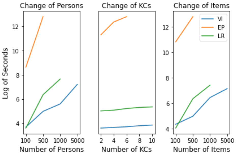
It is obvious to note that the results of the modified VI are better compared with that of the other methods in three aspects: (1) the computational speed of VI is faster as number of persons and items increase; (2) the modified VI gives better parameter estimation when the prior distributions disagree with the true distributions of the learning rates; (3) the modified VI supports real-time parameter estimations and requires less memories.

Real Data Study

In the third experiment, we used a real dataset, Riiid public dataset^[2] from Kaggle competition, to demonstrate the ability change tracking and answer prediction by OIRT.

We selected the event for a question being answered by the user (content_type_id=0) with prior question having explanation. We also removed the items and users with response frequencies fewer than 50. The data contained 6800 students, 1983 items and 146 KCs after preprocessing. We sorted the data by time the question was completed by the user, for ability tracking task, we used the whole data to estimate parameters; for answer prediction task, the first $90\%$ was used train models, and the remaining $10\%$ was used as testing set. We partition the data into 50 sessions with person-item pairs and feed one session into the model at a time.

We compared OIRT with XGBoost technique in answer prediction task. The reason for comparing with XGBoost is that both methods are single-layered and explainable models, which by nature are different and incomparable with the models based on deep neural networks. We only used ‘Timestamp’, ‘Tags’, ‘User ID’, and ‘Item ID’ as the input features for both OIRT and XGBoost. The ‘answered correctly’ was the label for the models. OIRT outperformed XGBoost in accuracy prediction of future question responses with limited input features: AUC=0.702 vs 0.689, ACC=0.733 vs 0.717 (since the XGBoost in the competition uses complex feature engineering, its AUCs reported in the competition are much higher). OIRT also provides reasonable estimates for user ability and item difficulty due to its high correlation with the observed accuracy proportion for students and items (0.751, 0.696, respectively).

We randomly selected 2 users and plotted Figure 2 to show the ability change tracking of OIRT by comparing with the observed differences of the accuracy proportion between two adjacent time points, averaging all KCs at each session. The estimations are equal to ($\overset{⃑}{\gamma_{i}^{s}} \odot \overset{⃑}{s_{i}} + \overset{⃑}{\gamma_{i}^{f}} \odot \overset{⃑}{f_{i}})^{T}\ \overset{⃑}{T_{j}}$ in Eq.3 at each time $t$ (below). The observed changes in accuracy proportion is equal to $\frac{{(\#\ correct\ KCs}_{1:t} - {\#\ correct\ KCs}_{1:t - 1})}{\#\ KCs}$ for each user (above), indicating how many more accurate KCs completed by a user at time $t$ relative to that at time $t - 1$.

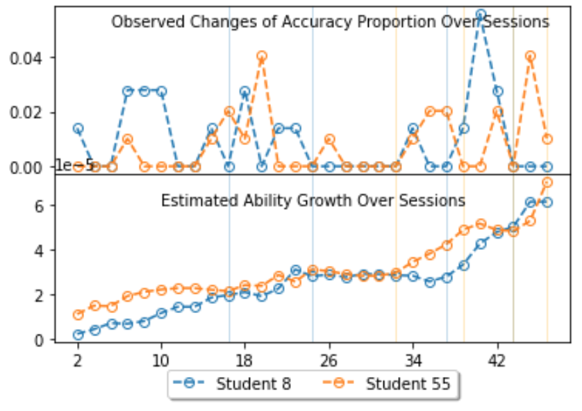
It can be seen when the observed increase in accuracy proportion are high between two adjacent time points, the estimated ability growth is more abrupt, such as sessions in the blue and orange windows for student 8 and student 55, respectively.

conclusions

In this study, we developed OIRT model and modified VI parameter estimation method to track student abilities in real-time and predict answer correctness for online learning system. Results show that the modified VI can estimate the parameters fast and effectively despite of the difference between the priors and the true distribution of the learning rate parameters.

Although OIRT performs relatively well in different tasks introduced above, it takes the form of generalized linear model, which has parameter identification issue and limits its performance in the accuracy prediction for future questions. We only predict answer accuracy based on historical data for individuals, and didn’t examine the prediction accuracy for new students, which will be explored more in future study.

REFERENCES

1. Albert, J. H. Bayesian estimation of normal ogive item response curves using Gibbs sampling. Journal of educational statistics, 17(3):251-269, 1992. https://doi.org/10.2307/1165149
2. Andrieu, C., N. De Freitas, Doucet, A., and Jordan, M. I. An introduction to mcmc for machine learning. Machine learning, 50(1):5–43, 2003.
3. Andrieu, C. and Thoms, J. A tutorial on adaptive mcmc. Statistics and computing, 18(4):343–373, 2008. https://doi.org/10.1007/s11222-008-9110-y
4. Cen, H., Koedinger, K., and Junker, B. Learning factors analysis–a general method for cognitive model evaluation and improvement. In International Conference on Intelligent Tutoring Systems, pages164–175. Springer, 2006. https://doi.org/10.1007/11774303_17
5. Curi, M., Converse, G. A., Hajewski, J., and S. Oliveira. Interpretable variational autoencoders for cognitive models. In 2019 International Joint Conference on Neural Networks (IJCNN), pages 1–8. IEEE, 2019. DOI:10.1109/IJCNN.2019.8852333
6. Hall, P., Johnstone, I., Ormerod, J., Wand, M., and Yu, J. Fast and accurate binary response mixed model analysis via expectation propagation. Journal of the American Statistical Association, 115(532):1902–1916, 2020. https://doi.org/10.1080/01621459.2019.1665529
7. Hambleton, R. K. and Cook, L. L. Latent trait models and their use in the analysis of educational test data. Journal of educational measurement, pages 75–96, 1977. http://www.jstor.org/stable/1434009.
8. Lord, F. A theory of test scores. Psychometric monographs, 1952. https://psycnet.apa.org/record/1954-01886-001
9. MacKay, D. J. The evidence framework applied to classification networks. Neural computation, 4(5):720–736, 1992. DOI: 10.1162/neco.1992.4.5.720
10. Martin, A. D., and Quinn, K. M. Dynamic ideal point estimation via markov chain monte carlo for the us supreme court. Political analysis,10(2):134–153, 2002. DOI: https://doi.org/10.1093/pan/10.2.134
11. Minka, T. Ep: A quick reference. Techincal Report, 2008.
12. Minka, T. P. Expectation propagation for approximatebayesian inference. arXiv preprint arXiv:1301.2294, 2013. https://doi.org/10.48550/arXiv.1301.2294
13. Park, J. Y., Cornillie, F., van der Maas, H. L., and Van Den Noortgate, W. A multidimensional irt approach for dynamically monitoring ability growth in computerized practice environments. Frontiers in psychology, 10:620, 2019. DOI: 10.3389/fpsyg.2019.00620
14. Patz, R. J. and Junker, B. W. A straightforward approach to markov chain monte carlo methods for item response models. Journal of educational and behavioral Statistics, 24(2):146–178, 1999. https://doi.org/10.2307/1165199
15. Pavlik Jr, P. I., Cen, H., and Koedinger, K. R. Performance factors analysis–a new alternative to knowledge tracing. Online Submission, 2009.
16. Rasch, G. Studies in mathematical psychology: I. probabilistic models for some intelligence and attainment tests. 1960.
17. Settles, B., Brust, C., Gustafson, E., Hagiwara, M., and Madnani, N. Second language acquisition modeling. In Proceedings of the NAACL-HLT Workshop on Innovative Use of NLP for Building Educational Applications (BEA). ACL, 2018. 10.18653/v1/W18-0506
18. Van der Linden, W. J. Handbook of item response theory: Volume 1: Models. CRC Press, 2016.
19. Van der Linden, W. J. and Jiang, B. A shadow-test approach to adaptive item calibration. Psychometrika, 85(2):301–321, 2020. doi: 10.1007/s11336-020-09703-8
20. Van der Linden, W. J. and Ren, H. A fast and simple algorithm for bayesian adaptive testing. Journal of educational and behavioral statistics, 45(1):58–85, 2020. https://doi.org/10.3102/1076998619858970
21. Wang, S. Expectation propagation algorithm, 2011.
22. Wang, S., Jiang, X., Wu, Y., Cui, L., Cheng, S., and Ohno-Machado, L. Expectation propagation logistic regression (explorer): distributed privacy-preserving online model learning. Journal of biomedical informatics, 46(3):480–496, 2013. doi: 10.1016/j.jbi.2013.03.008
23. Wang, X., Berger, J. O., and Burdick, D. S. Bayesian analysis of dynamic item response models in educational testing. The Annals of Applied Statistics, 7(1):126–153, 2013 https://doi.org/10.48550/arXiv.1304.4441
24. Wu, M., Davis, R. L., Domingue, B. W., Piech, C., and Goodman, N. Variational item response theory: Fast, accurate, and expressive. arXiv preprint arXiv:2002.00276, 2020. https://doi.org/10.48550/arXiv.2002.00276

1. Shrink controls the contribution of the KL terms in optimizing the loss function. Enhance gives more importance to KL terms as more data flows in, because the prior in KL at time $t$ contains the information from the previous data that we want to keep. Decay controls the weight given to the posterior at time $t - 1$ in contributing to the prior at time $t$. ↑

2. https://www.kaggle.com/c/riiid-test-answer-prediction/data ↑

© 2022 Copyright is held by the author(s). This work is distributed under the Creative Commons Attribution-NonCommercial-NoDerivatives 4.0 International (CC BY-NC-ND 4.0) license.