ABSTRACT
Student behaviour should correlate to the course performance. This paper explored different types of clustering algorithms using the pre-midterm student behaviour data. We found meaningful and interpretive results when clustering algorithms generate three clusters. The clusters can be briefly summarized as potential top performance (PTP) students, potential poor performance (PPP) students, and mixed performance (MP) students. We found that PTP students usually submit early and gain a high score, PPP students usually submit late and gain a low score, and MP students usually make most submissions. MP students are hard to cluster. However, we found a good connection between other students’ behaviour and performance if we leave out MP students.
Keywords
1. INTRODUCTION
Students expose different learning behaviours in programming courses. Several studies focused on analysing the students’ data in order to understand student behaviours [5, 1, 14, 11]. The clustering technique was one of the common methodologies used in such studies. There are several benefits to identifying students’ behaviours. First, groups of students with similar academic and behaviour characteristics would benefit from the same intervention, which can reduce the time for instructors to identify and implement the right intervention for individual students [12]. Second, a better understanding of students’ misconceptions can lead to a better support system for novice programmers and provide adaptive feedback for students [4]. Last but not least, it is also a common technique used to predict student performance [6, 20, 17].
Although clustering techniques can be a valuable tool for researchers to categorize different student behaviours, several studies only applied a single type of clustering algorithm in their experiments [4, 15, 3, 8]. However, clustering results can be affected by the wrong choice of the clustering algorithm, which can cause the result under the threat of validity. To address this issue, people should experiment with multiple clustering algorithms to confirm that different clustering algorithms produce similar results where the essential characteristics of the resulting clusters are identical. Our experiment confirms that clusters’ essential characteristics are the same across multiple clustering algorithms, forming further discussion foundations.
Many studies applied clustering techniques to predict student performances [10, 7, 16]. However, the data used in these studies generally include both the pre-midterm data and the post-midterm data. Because of a strong correlation between the midterm exam grades and the final exam grades [2, 6, 9], which is also true for our data (Pearson correlation of ), it suggests that students who failed the midterm are likely to fail the final exam. Therefore, it is critical to identify at-risk students before the midterm. Our study merged multiple clustering algorithms into a predictive model to predict students’ performance using pre-midterm data.
This study applied the clustering techniques to students’ behaviours exposed in their pre-midterm submissions in an auto-grading system, Marmoset [18], to categorize them into different clusters. We applied multiple clustering techniques and compared their results to remove any effects caused by the wrong choice of the clustering algorithm. Then we tried to predict students’ performance using these clustering techniques. The research questions we want to ask are:
- RQ1: Are different clustering algorithms producing different results?
- RQ2: What are the characteristics of students in different clusters?
- RQ3: What were the exam grades of students in different clusters?
We want to clarify that we want to separate RQ1 and RQ2 because RQ1 is closely related to the predictive power of the clustering techniques, while RQ2 mainly focuses on providing better insights into the clusters.
2. COURSE BACKGROUND
The data we used in the study is collected from an introduction-level programming course in an R1 university in Canada. Students were supposed to learn how to carry out operational tasks using the C and C++ languages, perform procedural and object-oriented programming, and other relevant programming knowledge. The preliminary experiments were based on the data of 130 students who attended both the midterm and final exams in the course. Programming knowledge was not required.
In the course, an auto-grading system, Marmoset [18], was used. We refer to a coding/programming question in Marmoset as a task. A task may contain multiple tests. For any task, a student can make multiple submissions against it. Marmoset will automatically test it for each submission and reveal some test results to the student. Students can thus learn some feedback from those test results and then improve or fix their code accordingly.
In the course, there were different types of coding questions. i) Coding Labs: coding labs took place in the lab room. There was exactly one assigned task for each coding lab, which was to be completed and submitted during the lab period ( hours in the morning). Before the midterm exam, the coding lab was scheduled weekly. After the midterm exam, the coding lab was scheduled biweekly. There was a corresponding extended deadline (the same date but in the evening). Some students may rely on that deadline rather than finish during the lab. ii) Homework Assignments: homework assignments were assigned for students to do at home. They were assigned during lab time. Before the midterm, homework problems were due the following week. After the midterm, homework problems were due approximately two weeks later. In every homework assignment, there were multiple tasks, all of which had the same deadline. iii) Coding Examination: there was an in-lab coding examination during the course. It was similar to a coding lab. However, its grade comprised a portion of the midterm grade. An extended deadline was also allowed for the coding examination.
3. EXPERIMENT AND RESULTS
3.1 Features
The auto-grading system Marmoset stored every student’s submission during the course. In our study, we extracted three features.
- passrate: for every Marmoset task, we calculated the best score (the best number of tests passed among the submissions) a student made before the task deadline. Then we divide the total number of tests of that task to form the passrate feature. Because every assignment had multiple tasks, so for assignments, we need to sum the tasks’ best scores to form the best score for an assignment, and we sum tasks’ total number of tests to form the total number of tests for an assignment. For example, assignment 1 had tasks and a total number of tests. If a student’s best submissions of that tasks passed , , , and tests separately, then the passrate of that student for assignment 1 will be . This process was not needed for coding labs since there was only one task in a coding lab. Table 1 shows the total number of tests for different assignments and coding labs.
- lastsub: we extracted the lastsub feature as how many minutes between the last submission a student made and the task deadline. If a student made any submission before the deadline, this feature would contain a non-zero value. Only if a student did not submit before the deadline can the value be zero. Note that this feature will be zero for students whose submissions met the extended deadline but did not meet the original deadline for coding labs.
- nsub: the nsub feature represents how many submissions a student made before the task deadline for a given task. For assignments, we summed the numbers of submissions of tasks to form the nsub of an assignment.
| assignment | # total tests | coding lab | # total tests |
|---|---|---|---|
| a1 | 54 | l1 | 8 |
| a2 | 85 | l2 | 19 |
| a3 | 73 | l3 | 19 |
| a4 | 87 | l4 | 19 |
The features used in clustering algorithms is summarized in Table 2.
| feature name |
|---|
| a_passrate |
| a_lastsub |
| a_nsub |
| l_passrate |
| l_lastsub |
| l_nsub |
3.2 RQ1: What are the clustering results from different clustering algorithms given the pre-midterm data?
For research question 1, we explored all types of the clustering algorithms provided in the scikit-learn python package [13]. It includes: K-Means (KM), Affinity Propagation (AP), Spectral Clustering (SC), Hierarchical Clustering (HC), and Density-based Spatial Clustering (DBSC). We standardize every feature by removing the mean and scaling to unit variance before clustering. For a sample , the standard score is calculated as:
where is the mean of the samples and is the standard deviation of the samples.
We tested different options for setting the number of clusters in different algorithms. We found that setting the number to will give us good interpretive results. In this section, we will only compare the labelling. For the characteristics of different clusters, we will discuss them in RQ2.
Table 3 presents the size of different clusters using different clustering algorithms. To compare the cluster results across different clustering algorithms, we used adjusted rand index [19] for evaluation. Random labelling samples will make the adjusted rand index close to , and the value will be exactly when the clustering results are identical. Table 4 presents the results. Note that a cluster may be given different labels in different clustering algorithms. We re-numbered them according to the findings in the discussion of RQ2.
| KM | AP | HC | SC | DBSC | |
|---|---|---|---|---|---|
| cluster 1 | 62 | 56 | 48 | 58 | 32 |
| cluster 2 | 59 | 65 | 75 | 63 | 89 |
| cluster 3 | 9 | 9 | 7 | 9 | 9 |
| first algorithm | second algorithm | adjusted rand index |
|---|---|---|
| KM | AP | 0.780665 |
| AP | SC | 0.730717 |
| KM | SC | 0.682500 |
| KM | HC | 0.557372 |
| HC | DBSC | 0.521486 |
| HC | SC | 0.515544 |
| AP | HC | 0.475727 |
| AP | DBSC | 0.414938 |
| SC | DBSC | 0.382402 |
| KM | DBSC | 0.322811 |
From Table 3 and Table 4, we can tell the clustering results from KM, AP, and SC are similar to each other (similar cluster sizes and high adjusted rand index value). In contrast, HC and DBSC produced different clustering results. Combining KM and DBSC should help reduce the effect of an improper pick of the clustering algorithms.
3.3 RQ2: What are the characteristics of students in different clusters?
We carefully examined students in different clusters. Interestingly, although the cluster results differed in the cluster size and the adjusted rand index metric, we found that students in different clusters share similar characteristics across different clustering algorithms. We name the students in the three clusters as: Potential-Top-Performance (PTP) students, Potential-Poor-Performance (PPP) students, and Mixed-Performance (MP) students.
Table 5 summarizes the characteristics of different students.
| PTP students | MP students | PPP students | |
|---|---|---|---|
| assignment passrate | |||
| assignment lastsub | days early | hours early | hours |
| assignment nsub | |||
| lab 1-4 passrate | lab 1,4: , lab 2: , lab 3: | ||
| lab 1 lastsub | hours early | hours early | minutes early |
| lab 2,3 lastsub | minutes early | minutes early | minutes early |
| lab 4 lastsub | minutes early | minutes early | minutes early |
| lab 1-4 nsub | lab 1,2,4: , lab 3: |
We also examined the students that were put into different clusters from different algorithms. In general, those students put into different clusters from different algorithms were those whose behaviour was in the middle of PTP students and MP students or the middle of PPP and MP students. However, we found there were no students put into the PTP cluster in one algorithm while being put into the PPP cluster in another algorithm. We can tell that students from these two clusters share no typical behaviour from any aspect.
3.4 RQ3: What were the exam grades of students in different clusters?
Because some students were put into different clusters from different clustering algorithms, we consider students in the PTP cluster only if they were put into the PTP cluster by all clustering algorithms. Similarly, students in the PPP cluster were only put into the PPP cluster by all clustering algorithms. The remaining students will be MP students.
In addition to the midterm grades and final exam grades, there was a coding examination grade, which will comprise a portion of the midterm grade. Figure 1 shows us the relation between the coding examination grades and different clusters. Figure 2 shows us the relation between midterm grades and final grades of different clusters.
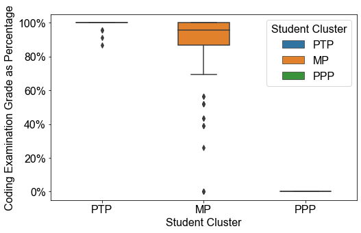
From Figure 1, we can see PTP students achieved a very high score on the coding examination, while PPP students achieved on the coding examination. The result is expected since PTP students mostly performed well on assignments and labs, which were programming questions. It is reasonable that they achieved a high score on the coding examination. In contrast, for PPP students, since they performed poorly on those questions, it is not surprising that they got a significantly low score.
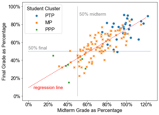
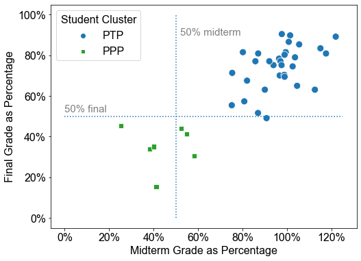
From Figure 2, we can see the performances of MP students messed up with other clusters of students. However, if we exclude them, as shown in Figure 3, we can see the performances of PTP students and PPP students were completely different. The reason we set a cut off point as for the exam grades is that it is the required grades for passing a course in the university.
It is essential to consider how many students genuinely need help from the identified PPP students. In other words, precision is important [2]. It is the higher, the better. Then we can calculate the precision of the PPP students, which is ( students out of the total PPP students were below in the midterm). Similarly, the precision of the final grades is , since no PPP students had a final grade above . These results are promising, implying that the clustering technique can predict student performance.
4. LIMITATIONS
The limitation of this study was that the data used in the study was of a limited amount. We appreciate any replicate studies to help validate the results in our study.
5. DISCUSSION
This study applied clustering techniques to pre-midterm students’ behaviour data by using an auto-grading system, namely how early students make their last submissions, how many submissions they make, and the best score. We found that different clustering algorithms label students differently and put them into different clusters, thus providing different predictive power. However, combining KM and DBSC clustering algorithms should help reduce the effect of an improper pick of the algorithms.
We found that the clusters share the same characteristics regardless of the labelling. We can summarize those clusters as Potential Top Performance (PTP) cluster, Potential Poor Performance (PPP) cluster, and Mixed Performance (MP) cluster (in which students might be put into different clusters from different clustering algorithms). We found that students in PTP/PPP are generally exposing behaviours at the extreme, and they perform well/poorly on the exams.
Better understanding the MP students is one of the future works. For example, whether there are sub-groups within this cluster, how to understand their learning behaviours, and what factors might prevent them from being successful in the course?
Although we are still at the preliminary stage, we believe our finding allows a fair evaluation of the participation of students in a course. Also, because our finding shows that predicting at-risk students in advance is possible, thus corrective actions to improve the final results might be implemented to help people achieve a learning environment with fairness and equity.
References
- M. An, H. Zhang, J. Savelka, S. Zhu, C. Bogart, and
M. Sakr. Are Working Habits Different Between
Well-Performing and at-Risk Students in Online
Project-Based Courses? In Proceedings of the 26th
ACM Conference on Innovation and Technology in
Computer Science Education V. 1, pages 324–330,
Virtual Event Germany, June 2021. ACM. ISBN
978-1-4503-8214-4. doi: 10.1145/3430665.3456320. URL
https://dl.acm.org/doi/10.1145/3430665.3456320. - H. Chen and P. A. S. Ward. Predicting Student Performance Using Data from an Auto-Grading System. In Proceedings of the 29th Annual International Conference on Computer Science and Software Engineering, CASCON ’19, pages 234–243, USA, 2019. IBM Corp. event-place: Toronto, Ontario, Canada.
- R. W. Crues, G. M. Henricks, M. Perry, S. Bhat,
C. J. Anderson, N. Shaik, and L. Angrave. How
do Gender, Learning Goals, and Forum Participation
Predict Persistence in a Computer Science MOOC?
ACM Transactions on Computing Education, 18(4):
1–14, Nov.
2018. ISSN 1946-6226. doi: 10.1145/3152892. URL
https://dl.acm.org/doi/10.1145/3152892. - A. Emerson, A. Smith, F. J. Rodriguez, E. N.
Wiebe, B. W. Mott, K. E. Boyer, and J. C.
Lester. Cluster-Based Analysis of Novice Coding
Misconceptions in Block-Based Programming. In
Proceedings of the 51st ACM Technical Symposium
on Computer Science Education, SIGCSE ’20,
pages 825–831, New York, NY, USA, 2020.
Association for Computing Machinery. ISBN
978-1-4503-6793-6. doi: 10.1145/3328778.3366924. URL
https://doi-org.proxy.lib.uwaterloo.ca/10.1145/3328778.3366924. event-place: Portland, OR, USA. - S. C. Goldstein, H. Zhang, M. Sakr, H. An, and
C. Dashti. Understanding How Work Habits influence
Student Performance. In Proceedings of the 2019
ACM Conference on Innovation and Technology
in Computer Science Education, pages 154–160,
Aberdeen Scotland Uk, July 2019. ACM. ISBN
978-1-4503-6895-7. doi: 10.1145/3304221.3319757. URL
https://dl.acm.org/doi/10.1145/3304221.3319757. - A. Hellas, P. Ihantola, A. Petersen, V. V. Ajanovski,
M. Gutica,
T. Hynninen, A. Knutas, J. Leinonen, C. Messom,
and S. N. Liao. Predicting academic performance: a
systematic literature review. In Proceedings Companion
of the 23rd Annual ACM Conference on Innovation
and Technology in Computer Science Education, pages 175–199, Larnaca Cyprus, July 2018. ACM. ISBN
978-1-4503-6223-8. doi: 10.1145/3293881.3295783. URL
https://dl.acm.org/doi/10.1145/3293881.3295783. - J.-L. Hung, M. C. Wang, S. Wang, M. Abdelrasoul,
Y. Li, and W. He. Identifying At-Risk Students
for Early Interventions—A Time-Series Clustering
Approach. IEEE Transactions on Emerging Topics
in Computing, 5(1):45–55, Jan. 2017. ISSN
2168-6750. doi: 10.1109/TETC.2015.2504239. URL
http://ieeexplore.ieee.org/document/7339455/. - H. Khosravi and K. M. Cooper. Using Learning
Analytics to Investigate Patterns of Performance
and Engagement in Large Classes. In Proceedings
of the 2017 ACM SIGCSE Technical Symposium
on Computer Science Education, pages 309–314,
Seattle Washington USA, Mar. 2017. ACM. ISBN
978-1-4503-4698-6. doi: 10.1145/3017680.3017711. URL
https://dl.acm.org/doi/10.1145/3017680.3017711. - S. N. Liao, D. Zingaro, K. Thai, C. Alvarado, W. G.
Griswold, and L. Porter. A Robust Machine Learning
Technique to Predict Low-Performing Students. 19(3):
1–19. doi: 10.1145/3277569. URL
https://doi.org/10.1145/3277569. - M. I. López, J. M. Luna, C. Romero, and
S. Ventura. Classification via clustering for predicting
final marks based on student participation in forums.
page 4. URL
https://eric.ed.gov/?id=ED537221. - K. Mierle, K. Laven, S. Roweis, and G. Wilson. Mining Student CVS Repositories for Performance Indicators. page 5, May 2005.
- S. Mojarad, A. Essa, S. Mojarad, and R. S.
Baker. Data-Driven Learner Profiling Based
on Clustering Student Behaviors: Learning
Consistency, Pace and Effort. In R. Nkambou,
R. Azevedo, and J. Vassileva, editors, Intelligent
Tutoring Systems, volume 10858, pages 130–139.
Springer International Publishing, Cham, 2018.
ISBN 978-3-319-91463-3 978-3-319-91464-0.
doi: 10.1007/978-3-319-91464-0_13. URL
http://link.springer.com/10.1007/978-3-319-91464-0_13. Series Title: Lecture Notes in Computer Science. - F. Pedregosa, G. Varoquaux, A. Gramfort, V. Michel, B. Thirion, O. Grisel, M. Blondel, P. Prettenhofer, R. Weiss, V. Dubourg, J. Vanderplas, A. Passos, D. Cournapeau, M. Brucher, M. Perrot, and Duchesnay. Scikit-Learn: Machine Learning in Python. 12:2825–2830. ISSN 1532-4435.
- V. Sher, M. Hatala, and D. Gašević. Analyzing
the consistency in within-activity learning patterns in
blended
learning. In Proceedings of the Tenth International
Conference on Learning Analytics & Knowledge, pages
1–10, Frankfurt Germany, Mar. 2020. ACM. ISBN
978-1-4503-7712-6. doi: 10.1145/3375462.3375470. URL
https://dl.acm.org/doi/10.1145/3375462.3375470. - D. B. Silva and C. N. Silla. Evaluation of students
programming skills on a computer programming
course with a hierarchical clustering algorithm. In
2020 IEEE Frontiers in Education Conference (FIE),
pages 1–9, Uppsala, Sweden, Oct. 2020. IEEE.
ISBN 978-1-72818-961-1. doi: 10.1109/FIE44824.2020.
9274130. URL
https://ieeexplore.ieee.org/document/9274130/. - S. Sisovic, M. Matetic, and M. B. Bakaric. Clustering
of imbalanced moodle data for early alert of student
failure. In 2016 IEEE 14th International Symposium on
Applied Machine Intelligence and Informatics (SAMI),
pages 165–170, Herlany, Slovakia, Jan. 2016. IEEE.
ISBN 978-1-4673-8740-8. doi: 10.1109/SAMI.2016.
7423001. URL
http://ieeexplore.ieee.org/document/7423001/. - S. E. Sorour, T. Mine, K. Goda, and S. Hirokawa.
A Predictive Model to Evaluate Student Performance.
Journal of Information Processing, 23(2):192–201,
2015. ISSN 1882-6652. doi: 10.2197/ipsjjip.23.192. URL
https://www.jstage.jst.go.jp/article/ipsjjip/23/2/23_192/_article. - J. Spacco, W. Pugh, N. Ayewah, and D. Hovemeyer.
The Marmoset project: an automated snapshot,
submission, and testing system. In Companion
to the 21st ACM SIGPLAN conference on
Object-oriented programming systems, languages,
and applications - OOPSLA ’06, page 669,
Portland, Oregon, USA, 2006. ACM Press. ISBN
978-1-59593-491-8. doi: 10.1145/1176617.1176665. URL
http://portal.acm.org/citation.cfm?doid=1176617.1176665. - D. Steinley. Properties of the Hubert-Arable
Adjusted Rand Index. Psychological Methods, 9
(3):386–396, 2004. ISSN 1939-1463, 1082-989X.
doi: 10.1037/1082-989X.9.3.386. URL
http://doi.apa.org/getdoi.cfm?doi=10.1037/1082-989X.9.3.386. - R. Venant, K. Sharma, P. Vidal, P. Dillenbourg, and
J. Broisin. Using Sequential Pattern Mining to Explore
Learners’ Behaviors and Evaluate Their Correlation
with Performance in Inquiry-Based Learning. In
Lavoué, H. Drachsler, K. Verbert, J. Broisin,
and M. Pérez-Sanagustín, editors, Data Driven
Approaches in Digital Education, volume 10474, pages
286–299. Springer International Publishing, Cham,
2017. ISBN 978-3-319-66609-9 978-3-319-66610-5.
doi: 10.1007/978-3-319-66610-5_21. URL
http://link.springer.com/10.1007/978-3-319-66610-5_21. Series Title: Lecture Notes in Computer Science.
© 2022 Copyright is held by the author(s). This work is distributed under the Creative Commons Attribution-NonCommercial-NoDerivatives 4.0 International (CC BY-NC-ND 4.0) license.