ABSTRACT

As computer-based learning platforms have become ubiquitous, there is a growing need to better support teachers. Particularly in mathematics, teachers often rely on open-ended questions to assess students’ understanding. While prior works focusing on the development of automated open-ended work assessments have demonstrated their potential, many of those methods require large amounts of student data to make reliable estimates. We explore whether a problem specific automated scoring model could benefit from auxiliary data collected from similar problems to address this “cold start" problem. We examine factors such as sample size and the magnitude of similarity of utilized problem data. We find the use of data from similar problems not only provides benefits to improve predictive performance by increasing sample size, but also leads to greater overall model performance than using data solely from the original problem when sample size is held constant.

Keywords

1. INTRODUCTION

The development of online learning platforms [12, 10] have transformed the instructional practices and learning experiences in traditional and expanded learning environments. These online-based learning platforms offer automated supports for assessing students’ work as well as providing feedback. While in the past these supports were generally restricted to closed-ended problems with a finite number of accepted correct responses, advancements in machine learning and natural language processing methods have led to the development of tools that support open-ended work [15, 4, 2]. As open-ended questions in mathematics are widely used by teachers to understand the students’ knowledge state and their understanding of a topic, these types of tools have great utility for both teachers and students using these systems.

Automatically scoring mathematical expressions and explanations has several distinctive challenges due to the interleaving of linguistic and non-linguistic terms (e.g. such as numbers and mathematical expressions). For example, [13] provides automatic grading and feedback for math open response questions using clustering techniques, but it ignores all text explanations to focus solely on numerical expressions. In the past few years, there have been several works focused on the development and improvement of automated methods for assessing student open-ended responses in mathematics [6, 18, 17, 8]. These methods are mostly based on evaluating given student answers based on historical student answers and the scores given by teachers to such data. [6] compared the performance of different models for scoring math open-ended responses and attempted to establish a benchmark evaluation procedure to evaluate future models. Building on that work, [2] improved performance by using Sentence-BERT (SBERT) [14] embeddings on the same dataset to score student responses. SBERT modifies the pre-trained BERT (Bidirectional Encoder Representations from Transformers) [5] model to generate sentence-level embeddings. Similar approaches are utilized in recommending feedback messages for teachers to give to students.

As is prevalent in several machine learning applications, many of these approaches are susceptible to the cold start problem, where implementations of such methods may lack sufficient data to make informed estimates. While the impact will vary depending on the model and the context, most assessment models require non-trivial amounts of data to make accurate predictions (c.f. [1]) which may take time and effort to acquire. In cases when there is a newer student response that has not been encountered in the past, these types of methods often fall behind in suggesting an accurate score/feedback message posing this as the cold start problem. In light of this, mitigating the impact of this cold start problem would provide support for teachers across a wider range of problems. Transfer learning [16] is commonly used as a means of addressing the cold start problem. Within the field of mathematics education, we may be able to leverage data from similar content to improve performance in cases where there would otherwise be insufficient data to train an automated assessment model.

We seek to explore the effectiveness of leveraging auxiliary data (student responses) to similar open-ended problems in the auto-scoring of a new problem with limited labeled data. With the goal of addressing the cold start problem, we intend to answer the following research questions: 1. Does the addition of new labeled data from a similar open-response problem, improve the predictive performance of single problem based auto-scoring models? 2. Does leveraging data from a similar problem lead to better model performance in comparison to using data from a randomly selected problem? 3. What is the effect of incorporating auxiliary data into the training of an auto-scoring model and are there any benefits beyond that of increasing sample size?

2. METHODOLOGY

2.1 Dataset

For this study, data¹ consists of all student answers that have ever been submitted to open-ended problems within ASSISTments. For this study, we arbitrarily selected an open response problem within this dataset that contained at least 40 student responses (n=45) to act as a representative problem. For consistency of terminology, this representative problem will be referred to as the “original problem” throughout this paper, and will represent the problem for which we would like to train an auto-scoring model (e.g. we will treat it as the problem with insufficient data).

The selected problem pertains to logarithms, and presents the students with the following equation: “$5\mathit{log}(x+4)=10$”; students are asked to either solve for $x$ and explain their steps to solve or to type “no solution” if no viable solution exists. We then collaborated with a content expert to select a similar open-ended problem with a comparable number of existing labeled student answers (n=43) to train a model. This second problem, referred to as the “similar problem” throughout the remainder of this paper, had the same prompt as the original problem but with the following equation: “$\mathit{lo}{g}_2(1-x)=4$”. While we acknowledge that the selected problems border on the threshold of what might be considered open-ended, much of the content of open curricula pair close-ended and open-ended components within many of their questions (e.g. solve and explain). In this way, the selected problems result in sufficient variation in student answers to examine auto-scoring models, and allow us to easily identify a problem with undeniable similarity both in terms of content and structure. As part of our analyses, we removed any problem from the remaining dataset containing fewer than 10 labeled student responses to mimic a practical application where such problems would not be considered sufficient in providing auxiliary data since we will be sampling from random problems.

Minor preprocessing was performed on the data to match the format of [2] which introduced the SBERT-Canberra model. These steps included the removal of HTML tags, other special characters, and references to images. Like in [6, 2], teacher-provided scores follow a 5-point integer scale ranging from 0, indicating poor performance, through 4, indicating high performance. While we acknowledge that ordinal relationships are lost by representing the labels in this way, the scale is converted to a 5-valued categorical one-hot encoded vector and modeled as a multi-class prediction task (i.e. the model treats each score as a mutually-exclusive label) to keep consistent with [2].

2.2 Model

The ’‘SBERT-Canberra” model [2] follows a similarity-ranking procedure to generate its predictions. When producing a prediction for a given student response, it applies SBERT to generate an embedding that captures semantic and syntactic meaning, such that similar responses are mapped to closer points within the embedding space. The SBERT embedding for this student response is compared to SBERT embeddings of historic labeled student responses. Using the Canberra distance measure [11], the score for the historic response corresponding to the smallest distance (i.e. the most similar response) is used as the score prediction. We chose to use this model as 1) it outperformed existing benchmarks in assessing student responses in mathematics [2], 2) no“training” involved in the traditional machine learning sense so we do not need to optimize hyperparameters, and 3) the model performance is directly linked to the scale and diversity of the historic responses.

2.3 Model Evaluation

To examine the use of auxiliary data, we conduct 2 analyses that each compare the SBERT-Canberra model with 3 different training sets. The analyses follow a bootstrapping procedure which samples with-replacement from the available data at increasing intervals. At each interval, student responses are randomly sampled to train and evaluate the model using 10-fold cross validation, where sampling is conducted within the training folds. This entire process is repeated 25 times, with the model performance being averaged across these iterations (to reduce noise caused by unlucky sampling). To evaluate the scoring results, the area under the curve, AUC, (calculated using the simplified multi-class calculation of ROC AUC from [9]) is used as the primary metric to compare the model’s predicted score of a student response to the actual score that was provided by a teacher.

The models are distinguished by their training data. The Baseline Model uses only student responses from the original problem. The Similar Problem Model uses a combination of student responses from the original problem as well as auxiliary responses sampled from the similar problem. Finally, the Random Problem Model uses a combination of student responses from the original problem as well as student responses sampled from 5 randomly-selected problems from the remaining dataset; per design and due to the scale of the data used, it is very unlikely for these problems to be similar to the original problem, allowing for comparisons to be made in regard to differing magnitudes of similarity.

We randomly sample 40 scored responses from the similar problem and from the 5 random problems to create a comparable set. Due to the large variations in sample sizes across problems within the dataset, we sample student responses for the Random Problem Model using a stratified selection method. From the 5 randomly-selected problems per interval, 8 scored student responses are randomly selected per iteration in the interval and they compose the 40 samples to supplement the training data from the original problem.

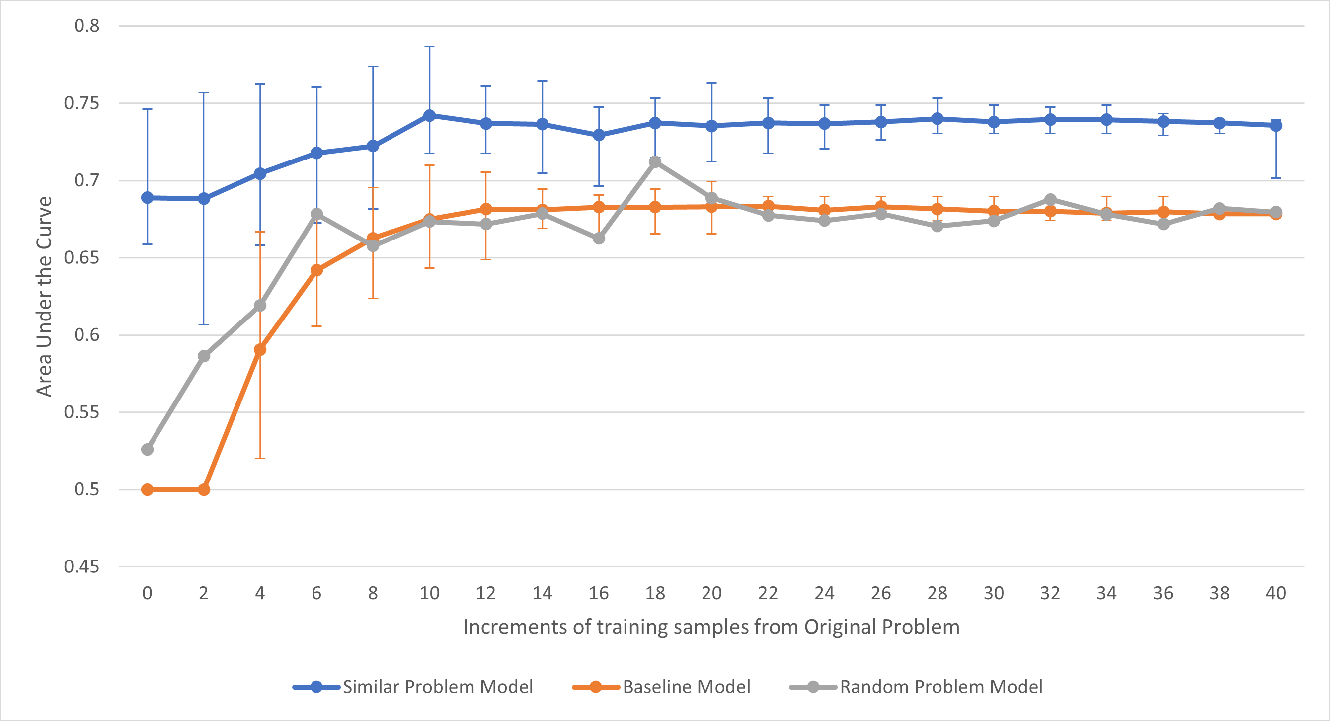
The first analysis replicates a real-world scenario where we may have a small number of labeled samples for the original problem, but a larger number of samples that may be leveraged from other problems. For each bootstrapping interval, we randomly sample data from the original problem ranging from 0 to 40. The average performance of each model is then plotted with 95% confidence intervals calculated over the 25 repeated runs per interval. While the Baseline model is limited to only the 0 to 40 original problem samples, both the Similar Problem Model and Random Problem Model are able to use 40-80 samples over the set of intervals.

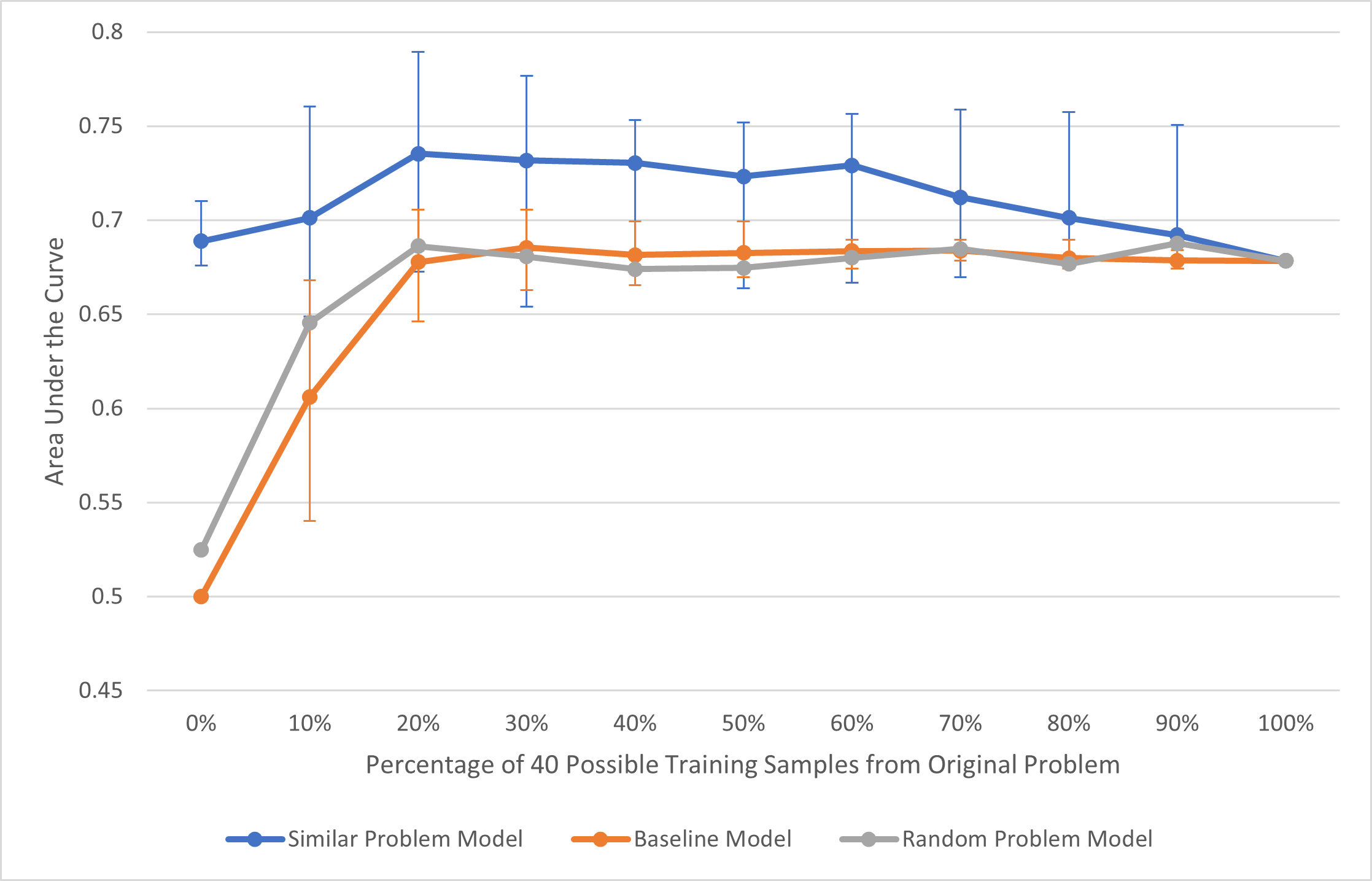
As it is hypothesized that the largest benefit of using auxiliary data is the added sample size, we conduct a second bootstrapping analysis that observes a constant sample size while varying the proportion of data used from the original problem. All models (except for the baseline) utilize 40 samples allowing us to see how the source of content affects model performance independent of data scale. The percentage intervals range from 0% to 100% of the training samples are from the original problem in 10% increments. So, at the first interval, all samples are responses from other problems, while at the end, all 40 samples are from the original problem. As the Baseline Model only utilizes data from the original problem, we are unable to maintain a consistent sample size across intervals. For comparative purposes, we increase the training sample size with the increasing percentage (i.e. using 0 samples, then 4 corresponding with 10%, etc.).

3. RESULTS AND DISCUSSION

For intervals 0 and 0%, no training data was provided for the baseline model so the average AUC of the baseline model is assigned to be 0.5 which is equivalent to chance.

Observing the Similar Problem Model in Figure 1, the model outperforms the average AUC of the baseline model across every increment of training samples from the original problem by approximately 0.073 in terms of average AUC per interval. This difference is also statistically reliable across a majority of intervals by comparing the confidence intervals.

Regarding the Random Problem Model, the model outperforms the average AUC of the baseline model across 43% of the increments tested. At an average difference of just 0.007 in terms of average AUC per interval, very little difference is observed between the Random Problem Model and the Baseline Model. It is worth noting that the performance of the Random Problem Model does outperform the Baseline over the initial intervals when sample size is the smallest, suggesting that even randomly-selected problems may provide benefit. However, this model also exhibited large variations in performance, leading us to omit the error bars to improve the readability of the figure; this variation is presumably attributable to the random selection of problems with varying magnitudes of similarity to the original problem.

An interesting trend emerged in regard to the Similar Problem Model as seen in Figure 2. When using 40 total training samples (and keeping this constant) with some percentage of samples from the original problem and the remaining samples from the similar problem, the modified model outperforms or equals the average AUC of the baseline model across every increment of training samples from the original problem by around 0.053 in terms of average AUC per interval. After the peak performance in terms of average AUC, the model’s performance lessens as the percentage of training samples coming from the original problem increases.

The Random Problem Model follows closely with the performance of the baseline. When using 40 total training samples with some percentage of samples from the original problem and the remaining samples from 5 random problems, the modified model outperforms or equals the average AUC of the baseline model across 54% of the increments tested and by around 0.005 in terms of average AUC per interval.

The Baseline Model across both analyses provide insights into the current implementation of auto-scoring models. While the performance of the SBERT-Canberra model will likely vary across problems, we observe here that the model converges within a relatively small set of samples. After training from 12 samples from the original problem, the baseline model converges in terms of average AUC performance. It does seem to matter, however, which samples are used to train the model. We can see in both analyses that the Baseline Model’s confidence intervals decrease with more samples. The relatively wide bounds over low sample sizes suggests that there are subsets of training samples that are better than others. This is not surprising as the diversity of data is often considered just as important as the scale in many machine learning applications [7].

There is a similar trend in regard to the scale of confidence bounds for the Similar Problem Model. Although the average AUC performance stabilized after 10 samples, the confidence intervals continued to shrink in the first analysis, but remained relatively constant in the second analysis. In both analyses, however, we see consistent, if not statistically reliable differences in comparison to the Baseline Model. In addressing our first research question, this finding suggests that the use of auxiliary data can lead to notable benefits to model performance. We see in the first analysis that the added sample size leads to notable performance through all intervals. While our initial hypothesis was that this benefit would likely be attributable to increased sample sizes, the trend of this Similar Problem Model in the second analysis contradicts that hypothesis. While this model still outperforms the baseline, as sample size is held constant, this cannot be the contributing factor to the differences we observe. We expected the final interval of Figure 2 to be an upper bound for model performance as this is when the data is most closely related to the test set, but we found that the inclusion of data from a similar problem added benefits that extend beyond the impact of sample size. This finding addresses our third research question, but still remains inconclusive as to what benefit is provided. It is possible, for example, that the auxiliary data acts as a regularization method (c.f. [3]), but the analyses conducted here are only able to rule out sample size being the contributing factor. These findings further confirm that scoring models can be improved upon when provided with more varied training samples from both the problem it is trying to score and similar problems rather than only being trained from samples of the original problem. Even when trained with the same number of samples, the Similar Problem model’s average AUC decreases after a peak training percentage composition which supports the theory that the quality of the training samples from the original problem are less than the quality of the combined samples.

What is perhaps most surprising about this comparison in the second analysis is that the model trained from 100% of data from the similar problem seems to outperform the model trained from 100% of the original problem. We believe that this is an artifact of the selected problems and the level of similarity that they exhibit. As such, we would not expect this finding to extend to every open-ended problem, but rather could extend to a subset where there is strong similarity between problems both in terms of content and the structure of student responses; this is the scenario where we believe this method would provide the most benefit.

This is particularly the case considering that the same level of benefit was not observed in regard to the Random Problem Model across the two analyses. Our hypothesis, as previously introduced, is that the added benefit is likely correlated with the magnitude of problem similarity. Even if this hypothesis is flawed, we are seeing that certain subsets of problems lead to better performance than others, emphasizing the importance in selecting suitable problems from which to draw auxiliary data. In light of this, we can address our second research question in that problem similarity, loosely defined, does seem to impact performance.

4. CONCLUSIONS AND FUTURE WORK

In this paper, we explore a possible solution to the cold-start problem in automating the assessment of student open-ended work. We have shown that our SBERT-Canberra method using similar auxiliary problem data consistently and significantly outperformed the model using data solely from the original problem. When there are few training samples, even the modified SBERT-Canberra method using random problems’ data to supplement helped improve the performance. Throughout the exploration of both analyses, there is a noticeable benefit to supplementing the training samples with data from other problems. By supplementing the original training samples with multiple similar problems, we hypothesize that it will lead to even larger performance improvements to automatic scoring regardless of the number of original training samples. This would be particularly the case if our hypothesis is correct where some of this benefit is derived from regularizing factors.

The largest limitation is that this paper focuses on predicting the scores of only one specific problem. While we argue that the analyses conducted here were sufficient to address our research questions, there is a larger uncertainty that remains in regard to how representative these results are. This work should be tested across a variety of problems to ensure that the results generalize well to other problems. When deciding what constitutes a similar problem, future work could explore other methods that consider a wide range of comparison characteristics. Descriptives including the problem text, knowledge component, grade level, average difficulty, etc may be utilized in comparing problems to determine similarity. Defining such attributes would also provide opportunities to build models to better understand how matching characteristics correlate with model performance gains.

Future work should use transfer learning to use the SBERT-Canberra model of a similar problem as a starting point to score a new problem’s open-ended response. As more data from problems are collected, we found that there may still be benefits to using auxiliary data even beyond addressing the cold start problem. Furthermore, teachers often need supports in providing more meaningful feedback beyond that of a numeric score. ASSISTments is already able to recommend feedback for trained problem models, but it requires a lot of data in order to do so (more than for the automated scoring task). The use of auxiliary data as explored in this work may prove useful in other such contexts.

5. ACKNOWLEDGMENTS

We thank multiple NSF grants (e.g., 1917808, 1931523, 1940236, 1917713, 1903304, 1822830, 1759229, 1724889, 1636782, 1535428, 1440753, 1316736, 1252297, 1109483, & DRL-1031398); IES R305A170137, R305A170243, R305A180401, R305A120125, R305A180401, & R305C100024, the GAANN program (e.g., P200A180088 & P200A150306 ), and the EIR, ONR (N00014-18-1-2768), Schmidt Futures and a second anonymous philanthropy.

6. REFERENCES

1. M. Banko and E. Brill. Scaling to very very large corpora for natural language disambiguation. In Proceedings of the 39th annual meeting of the Association for Computational Linguistics, pages 26–33, 2001.
2. S. Baral, A. Botelho, J. Erickson, P. Benachamardi, and N. Heffernan. Improving automated scoring of student open responses in mathematics. In Proceedings of the Fourteenth International Conference on Educational Data Mining, Paris, France, 2021.
3. J. Bouwman. Quality of regularization methods. DEOS Report 98.2, 1998.
4. S. A. Crossley, K. Kyle, and D. S. McNamara. The tool for the automatic analysis of text cohesion (taaco): Automatic assessment of local, global, and text cohesion. Behavior research methods, 48(4):1227–1237, 2016.
5. J. Devlin, M.-W. Chang, K. Lee, and K. Toutanova. Bert: Pre-training of deep bidirectional transformers for language understanding, 2019.
6. J. A. Erickson, A. F. Botelho, S. McAteer, A. Varatharaj, and N. T. Heffernan. The automated grading of student open responses in mathematics. In Proceedings of the Tenth International Conference on Learning Analytics & Knowledge, pages 615–624, 2020.
7. H. J. Hadi, A. H. Shnain, S. Hadishaheed, and A. Ahmad. Big data and five v’s characteristics. 2014.
8. G. Haldeman, M. Babeş-Vroman, A. Tjang, and T. D. Nguyen. Csf: Formative feedback in autograding. ACM Transactions on Computing Education (TOCE), 21(3):1–30, 2021.
9. D. J. Hand and R. J. Till. A simple generalisation of the area under the roc curve for multiple class classification problems. Machine Learning, 45:171–186, 2001.
10. N. T. Heffernan and C. L. Heffernan. The assistments ecosystem: Building a platform that brings scientists and teachers together for minimally invasive research on human learning and teaching. International Journal of Artificial Intelligence in Education, 24(4):470–497, 2014.
11. G. Jurman, S. Riccadonna, R. Visintainer, and C. Furlanello. Canberra distance on ranked lists. In Proceedings of advances in ranking NIPS 09 workshop, pages 22–27. Citeseer, 2009.
12. K. R. Koedinger, A. Corbett, et al. Cognitive tutors: Technology bringing learning sciences to the classroom. na, 2006.
13. A. S. Lan, D. Vats, A. E. Waters, and R. G. Baraniuk. Mathematical language processing: Automatic grading and feedback for open response mathematical questions, 2015.
14. N. Reimers and I. Gurevych. Sentence-bert: Sentence embeddings using siamese bert-networks, 2019.
15. R. D. Roscoe and D. S. McNamara. Writing pal: Feasibility of an intelligent writing strategy tutor in the high school classroom. Journal of Educational Psychology, 105(4):1010, 2013.
16. L. Torrey and J. Shavlik. Transfer learning. In Handbook of research on machine learning applications and trends: algorithms, methods, and techniques, pages 242–264. IGI global, 2010.
17. X. Yang, L. Zhang, and S. Yu. Can short answers to open response questions be auto-graded without a grading rubric? In International Conference on Artificial Intelligence in Education, pages 594–597. Springer, 2017.
18. L. Zhang, Y. Huang, X. Yang, S. Yu, and F. Zhuang. An automatic short-answer grading model for semi-open-ended questions. Interactive learning environments, 30(1):177–190, 2022.

© 2022 Copyright is held by the author(s). This work is distributed under the Creative Commons Attribution-NonCommercial-NoDerivatives 4.0 International (CC BY-NC-ND 4.0) license.