* These two authors made the same contribution.
† The corresponding author.

ABSTRACT

Attendance reflects students' study motivation, and serves as an important indicator in educational management. A strong correlation has been found between attendance and academic performance. Due to the time varying nature of attendance and the challenge of collecting data automatically, few studies explored the longitudinal attendance of student subpopulations. In this paper, we introduce a new method combining Exponential Moving Average (EMA) and Kullback-Leibler Divergence (KLD) to identify longitudinal attendance patterns. We justify that KLD best preserves the structural difference between attendance distributions in student subpopulations. Using real-life data from a university, our result identifies the critical period when high and low academic performance students diverge in attendance, which calls for the attention of educators.

Keywords

INTRODUCTION

Attendance is an important indicator in education. It interplays with many other factors, such as instructional quality, psychological status, and academic performance which lies in the essence of education. Many studies confirmed the correlation between attendance and attainment, using methods including hypothesis test [20], correlation analysis [1] and prediction [32, 33]. Furthermore, many studies identified positive relation between drop out and low attendance [12, 30]. These studies suggest that attention data provides valuable information in the early detection and assistance of students with low attendance. However, few studies considered associating longitudinal attendance data with academic performance.

Longitudinal attendance data reveals the dynamics between attendance and academic success, but is still under-researched. Though many educators are aware of the importance of attendance and have carried out certain attendance policy, the lack of deep understanding of the interaction between attendance and academic success hinders the design and implementation of effective attendance policy. This is especially true for universities, where a mandatory attendance policy on every course at all time is usually not pervasive.

With the popularity of smart devices and the arrival of Internet of Things (IoT), longitudinal attendance data can be collected automatically and in a large scale. Techniques such as Bluetooth/Beacon [2, 31], face recognition [13] and Wi-Fi tracing [23, 34] have been applied to detect attendance automatically. [7] collected attendance data in an institution-wide fashion. The abundance of data makes it easier to study longitudinal attendance, and calls for new methods and in-depth analysis.

Traditionally longitudinal attendance data is assessed by simple statistics and line charts. The average attendance rate over a period of time (e.g., a week or a semester) is a widely adopted indicator of students’ attendance. While being effective in many educational applications, a single average value is subject to noise in the period. For example, in attendance data collected using Wi-Fi tracing [7, 23, 34], the mal-function of some access points on campus can lead to inaccurate weekly attendance data for students. When studying the weekly attendance data in a time series, the fluctuation of data points can lead to wrong interpretation of the trend in attendance.

The comparison of the attendance for two student populations is another challenge. For example, it is interesting to compare the trends of attendance for students with top 25% and last 25% academic performance. However, the handy line chart of weekly average attendance rates does not fully reflect the structure inside each population.

Below we list the research questions of this study.

1. How to measure attendance dissimilarity from the fluctuating attendance time series between student subpopulations with different academic performance?
2. What can we learn from the divergence of attendance patterns for students with different academic performance?

For Question 1, when measuring the dissimilarity between two populations, in order to preserve as much information in the student populations as we can, we apply Kullback-Leibler divergence (KLD) on attendance data. KLD was first introduced in 1951 by Kullback and Leibler [18]. It was proposed as a measure of dissimilarity between statistical populations in terms of information. We will show below that comparing with other commonly used methods, KLD emphasizes more on inner structural divergence between the attendance data of student populations with different academic performance.

To deal with fluctuation, we propose to apply Exponential Moving Average (EMA) to smooth the time series in order to obtain trend and regional information. Moving average is a simple but widely adopted technique in time series analysis, and has been applied to process longitudinal data in many areas. Learning from the successful application of exponential moving average methods on implementing weekly stock index [9], we apply it on weekly attendance index calculation.

For Question 2, we propose the combination of Exponential Moving Average and KLD to detect critical periods when attendance patterns of students with top 25% and last 25% academic performance diverge dramatically.

In summary, the contributions of this study are as follows. We propose to apply the combination of Exponential Moving Average (EMA) and Kullback-Leibler divergence (KLD) to study longitudinal attendance data. So far as we know, there is no previous study that apply EMA or KLD on attendance data. We derive random subsamples to study moving average indexes and dissimilarity functions of student populations. Experiment results on attendance data shows that our method out-performs traditional methods. The application of our method on first year university students shows that the attendance of the top 25% and last 25% students on academic performance diverges during mid-term periods and holidays, which calls for the attention of university managements.

The rest of this paper is organized as follows. Section 2 describes the related studies. Section 3 introduces our method. Section 4 presents the results. Section 5 describes the limitations. Section 6 draws the conclusions.

RELATED STUDIES

The time variant nature of attendance contains rich details for student behaviors changes; however, before attendance data can be collected automatically, attendance is usually collected by signup sheets which have to be process manually and hinder the study of longitudinal attendance data. [6, 21] observed declines in student attendance over the duration of academic years. [12, 27] treated students’ attendance as time series data and performed clustering. [32] studied the life-cycles of 48 students using multiple dimensions of data, including raw attendance data from GPS tracing and Wi-Fi tracing. Valuable information was collected from these results.

Critical period detection is often associated with time series analysis. [11] divided students into several bands according to their academic performance, plotted the cumulative credit time series of each student subpopulation and detected divergent critical points using unpaired t-test. [29] identified students’ withdrawal routes by showing the proportion of students not submitting their assignments and found that only very few of them returning to submit the next ones. [4] researched into MOOC data, plotted students’ activity time series and found activity peaks before each assessment due. None of these researches considered attendance time series. Using attendance records from high schools in New York, [16, 17] found weekly cycles and detected abnormal data points. The authors [15] then utilized the results to identify problems and provide suggestion for high school educators. These researches considered attendance, but did not associate it with academic performance.

Kullback-Leibler Divergence (KLD) is a popular method to calculate the difference between two populations. It has been justified as a sensitive dissimilarity measurement for probability distribution [35]. In the context of education, KLD is widely applied to detect test collusion by comparing unusual distribution of individual testing behavior to that of the whole test taker population [3, 19]. Besides, KLD was applied in [8, 26, 28] to classify students into groups by maximizing the divergence of certain quality between distributions of different subpopulations. [24] observed student’s learning trajectory by calculating the difference between quizzes data collected before and after instructions. So far as we know, there is no previous study that applied KLD to attendance data of student populations.

Moving Average (MA) method is one of the most popular techniques in time series analysis. It’s often used for the purpose to smooth and track the trend in longitudinal data [9]. Exponential Moving Average, as a variation of Moving Average, is widely used in many area, including finance [9, 10], sales analysis[14], weather forecasting[5] and education [25] (to predict enthusiasts in mathematics programs). So far as we know, no previous study has applied exponential moving average on attendance data.

METHOD

Data and Setup

Anonymous data of students’ cumulative GPA (denoted as CGPA) and attendance data were retrieved from a university in China with approval from the university management. The data was collected from undergraduate students spanning over 3 semesters in 2018 and 2019, namely, Fall 2018, Spring 2019 and Fall 2019 (noted that academic year starts in a Fall semester). To protect privacy, student IDs were converted into hash code beforehand.

For most courses, students received letter grades from A to F. As an example, only 15 out of 426 courses taught in academic year 2018 are courses with P/F grades. These courses were mostly for internship or research methodology/seminar, which were seldom taken by undergraduates in their first two years of study. All courses with P/F grades were excluded in calculation.

Attendance data was collected using a Wi-Fi based method and was handled using method proposed in [23, 34]. Students’ weekly attendance rate was calculated by taking the average of attendance within a week. For most courses, no mandatory attendance policy was established. The rest of courses that declared mandatory attendance policy were mostly university core courses which should be taken by all undergraduates.

Moving Average Index

In this subsection, we introduce exponential moving average methods to smooth the attendance curve.

Let $a_{i,t}$ be the attendance rate at time $t$ for student $i$, then we have $a_{i,t} \in \lbrack 0,\ 1\rbrack$. Let $\text{EMA}_{i,t}$be the corresponding index for student $i$ at time $t$. Exponential moving average can be calculated using the formulas below.

Definition 1 Exponential Moving Average (EMA):

$$\text{EMA}_{i,t} = \left\{ \begin{matrix} a_{i,1\ }\ \ \ \ \ \ \ \ \ \ \ \ \ \ \ \ \ \ \ \ \ \ \ \ \ \ \ \ \ \ \ \ \ \ \ \ \ \ \ \ \ for\ t = 1 \\ \beta a_{i,t} + \left( 1 - \beta \right)\text{EMA}_{i,t - 1}\ for\ t > 1 \\ \end{matrix} \right.\$$

$\beta$ stands for the weighting decay factor taken between 0 and 1. Commonly it’s set to be $\beta = 2/(n + 1)$ with $n = 2$ in our experiment (see the appendix for details).

EMA assigns the highest weight for the most recent data. The weight for the earlier data points decay with time via recursive process. Therefore, the earliest data would never vanish in the process of gaining successive values.

Dissimilarity Measurement

In this subsection, we study the dissimilarity measurements between attendance data of two student populations. Ideally, we want to find a dissimilarity measurement that can best reflect inner structure divergence between the two concerned populations.

Definition 2 Mean Difference (MDF): Let $a_{i,t}$ be the attendance rate at time $t$ for student $i$. Let P and Q be two distributions of $a_{i,t}$ at time $t$ of two populations of students. The mean difference (MDF) of P and Q is calculated as below.

$$MDF(P,Q) = \ E\left( P \right) - E(Q)$$

MDF is the simplest way to measure difference between two population. However, this measurement ignores the inner structure of distributions.

Definition 3 Absolute Distance (AD) & Definition 4 Kullback-Leibler Divergence (KLD): We divide the domain of distributions P and Q into several attendance intervals and name these intervals 1, 2, …, $n$. Then the probability of a student from distribution $\text{P\ }\text{or}\text{\ Q}$ falling in a given interval is $p_{1},p_{2},\ldots,p_{n}\ \text{or}\ q_{1},q_{2},\ldots,q_{n}$. We calculate the absolute distance (AD) and KLD as follows.

$$\text{AD}\left( P,Q \right) = \sum_{j = 1}^{n}{|p_{j} - q_{j}|}$$

$$\text{KLD}\left( P,\ Q \right) = \sum_{j = 1}^{n}{p_{j}log(\frac{p_{j}}{q_{j}})}$$

Both AD and KLD consider the inner structures of the distributions [35]. However, KLD is more sensitive when detecting inner structure differences than absolute distance.

The difference between AD and KLD can be illustrated by an example as follows. Let $A,\ B1,\ B2$ be three student populations. Divide the domain evenly into 4 intervals based on the attendance rates of the students: last 25% quantile, 25% - 50%, 50% - 75%, top 25% quantile. Probability of the three populations fall into the above-mentioned intervals are listed below. For example, 0.25 represent 25% of the population.

A: [0.25, 0.25, 0.25, 0.25]

B1: [0.30, 0.30, 0.30, 0.10]

B2: [0.40, 0.25, 0.25, 0.10]

For A, the attendance rates of students are evenly distributed in the 4 intervals. B1 differs from A by moving 15% of the population from the top quarter to the other 3 intervals evenly. B2 differs from A by moving 15% of the population from the top quarter to the last quarter only. Therefore, A overall should be considered to have higher attendance than B1 and B1 higher than B2.

Calculate the dissimilarity between A and B1, A and B2 using AD and KLD respectively, we have

$$\text{AD}\left( A,\ B1 \right) = AD\left( A,\ B2 \right) = 0.3$$

$$\text{KLD}\left( A,\ B1 \right) = \ 0.072,\ KLD\left( A,\ B2 \right) = 0.096$$

$$\text{KLD}\left( A,\ B2 \right) > KLD(A,B1)$$

In this example, AD cannot distinguish the difference between B1 and B2 in terms of the dissimilarity to A, while KLD correctly measures the dissimilarity order. It illustrates that KLD is more sensitive to inner structure differences than AD. MDF is not calculated in this example because we do not have the detailed distribution. In the result section, we will demonstrate the advantage of KLD over MDF and AD using random subsamples derived from real-life data.

RESULTS

Dissimilarity Measurement Selection

We make comparisons of dissimilarity measurements using large samples of random groups synthesized from our dataset. Though this experiment, we want to show that KLD can best illustrate the difference in attendance data between top students and other students.

Attendance data used is collected from students from Cohort 2018 in Fall 2018 and Spring 2019 semesters. We consider students’ overall attendance rates in the academic year 2018-19. We use their first year CGPA as the measurement of academic performance.

There are 120 students whose academic performance are in top 10%. Therefore, we set the top 120 students as top 10% group and randomly generate 10000 groups, each of 120 randomly selected students from the whole student population.

We divide the whole student population evenly into 4 levels based on their overall attendance rates. In each level there are 25% of students from the whole population. we then calculate for each group, the portion of students in each level. For example, for top 10% group, its attendance rate distribution in the 4 levels (from low to high) is: [0.125, 0.242, 0.3, 0.333]

We perform the three candidate dissimilarity measurements between the 10000 groups and the top 10% group. Noted that for KL-divergence, the direction is from the top 10% group to the generated group. We then find out the 3 groups (named as KLD, AD, MDF) having the largest attendance dissimilarity via the 3 different measurements and rank the 3 groups’ academic performance among the 10000 groups. Intuitively, the group with the largest difference from the top 10% group have the poorest academic performance.

The results are shown in Table 1. The rankings of mean GPA and the last 10% ratio indicate the academic performance of the chosen group among the 10000 groups (the higher the ranking the poorer the academic performance). We can see that the group detected by KLD has the highest mean GPA rank (last 1) among 10000 groups and the highest last 10% ratio rank (last 328) among the three dissimilarity measurements. Therefore, KLD is a good dissimilarity measurement and we apply it for distribution comparison on attendance difference.

For more experiment of dissimilarity measuerment selection, please see the appendix.

Exponential Moving Average and KLD

In this subsection, we compare the performance of two methods, KLD combined with EMA (denoted as EMA+KLD) and KLD combined with the raw attendance rates (denoted as RAW+KLD). The partition of data and the experiment setup are similar to those in section 4.1.

The results are shown in Table 2. The group detected by EMA combined with KLD has a higher mean GPA rank (last 24) and a higher last 10% ratio rank (last 276) than the group detected by Raw+KLD. Therefore, combining exponential moving average and KLD improves our ability to detect attendance divergence betweem student subpopulations of different academic performance.

For more information of EMA, please see the appendix.

Critical Periods in Attendance Divergence

In this subsection, we discuss the longitudinal attendance divergence between top and last 25% students on CGPA. The data is collected from first year undergraduate students in Fall 2018 and Spring 2019.

Figure 1 shows the KLD time series calculated between attendance of top and last 25% students using weekly attendance indexes processed with EMA. Noted that for KLD, we calculated the distance in the direction from the top population to the last population. The top and last quarter students first diverge after the 3-days national holiday (Fall 2018 Week 4, the Mid-autumn festival). In the mid-term period, the difference enlarges again and the difference stays at about the same level till the end of the semester. At the beginning of Spring 2019 semester, the attendance difference is reduced but is restored to the level of the last term quickly. During the mid-term of Spring 2019, the difference is enlarged and stays at the same level till the end of the semester.

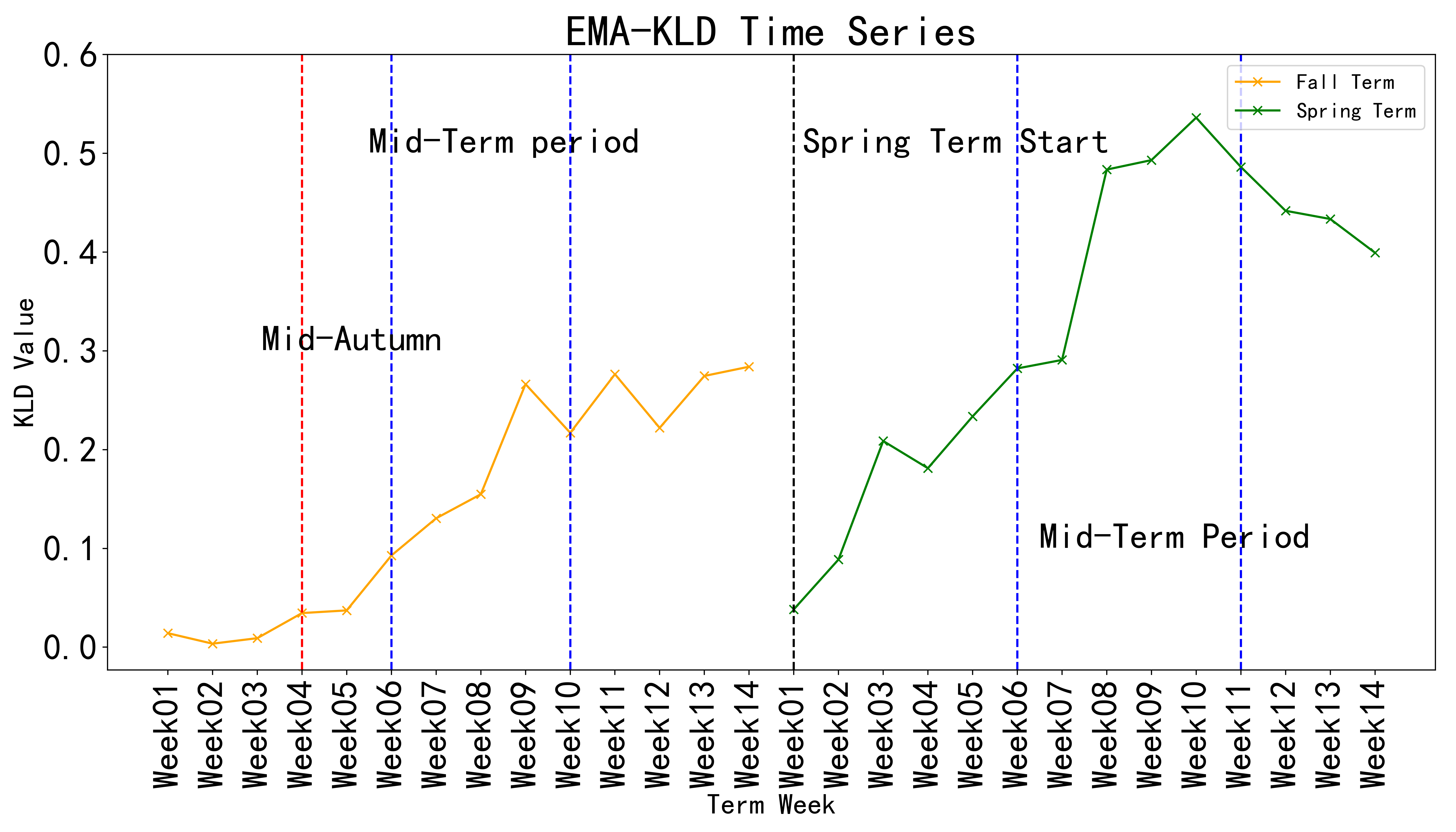
We conjecture several reasons behind the divergence of attendance rates. In the local culture, the 3-days national holiday (Mid-autumn festival) is the time when people travel to meet their love ones. Since the holiday is close in time to another national holiday, some students may leave the university and do not return to the university till the end of the second holiday. This behavior could lead to low attendance rates among the last quarter students during the week after the Mid-autumn festival. The mid-term period significantly enlarges the difference and multiple factors can be behind the phenomenon. The last quarter students could be frustrated by the mid-term exams and give up their studies; Preparing the mid-term exams is stressful and some students did not relax properly after the exams and start skipping classes; Some students might be addicted to video games and persistently reduce their class attendance.

Limitations

Raw attendance rate data used in our research was collected using a Wi-Fi based method proposed in [23, 34]. The data can be biased because some students would close their Wi-Fi connections or even close their digital devices all together, leading to a false label of absence. To avoid the possible bias, students whose data having less than 50 Wi-Fi connection records in a week were excluded. Previous studies [7, 22, 33] show that attendance collected from Wi-Fi tracing has usable accuracy. EMA can help reducing the noise and fluctuations in the attendance data.

Privacy is an importance issue in research related to Wi-Fi tracing. In our study, we removed personal information from the data and encrypted the student ID with a hash code. Attendance data and CGPA data were connected using this hash code. The Wi-Fi data collection had a clear location boundary and data was collected only when the students are on campus. We did not collect website URLs or communication content. Given that the research can potentially improve the existing attendance policy, this study has been approved by the university management.

CONCLUSIONS

In this study, we identified the divergence of longitudinal attendance patterns between student subpopulations of different academic performance using the combination of Exponential Moving Average (EMA) and Kullback-Leibler Divergence (KLD).

We designed several experiments to prove the efficacy of EMA and KLD to process raw attendance data and measure dissimilarity between top and last student populations. We then combined EMA and KLD to analyse real-life attendance data from two student subpopulations of top and last academic performance. The resulting curves are intuitive and imply rapidly increasing attendance divergence during the mid-term periods and right after public holidays.

Through the visualized results generated using our proposed method, we address the importance of longitudinal attendance patterns on academic performance. Our result gave educator an example on how to measure longitudinal attendance and can potentially help institutes to optimize attendance policy.

ACKNOWLEDGEMENTS

This work was supported by Shenzhen Research Institute of Big Data.

REFERENCES

1. Alexander, V. and Hicks, R.E. 2016. Does class attendance predict academic performance in first year psychology tutorials. International Journal of Psychological Studies. 8, 1 (2016), 28–32. DOI:https://doi.org/10.5539/ijps.v8n1p28.
2. Avireddy, S., Veerapandian, P., Ganapati, S., Venkat, M., Ranganathan, P. and Perumal, V. 2013. MITSAT — An automated student attendance tracking system using Bluetooth and EyeOS. Proceedings of 2013 International Mutli-Conference on Automation, Computing, Communication, Control and Compressed Sensing (iMac4s) (2013), 547–552.
3. Belov, D.I. 2013. Detection of Test Collusion via Kullback–Leibler Divergence. Journal of Educational Measurement. 50, 2 (2013), 141–163. DOI:https://doi.org/10.1111/jedm.12008.
4. Breslow, L., Pritchard, D.E., DeBoer, J., Stump, G.S., Ho, A.D. and Seaton, D.T. 2013. Studying learning in the worldwide classroom research into edX’s first MOOC. Research & Practice in Assessment. 8, (2013), 13–25.
5. Cadenas, E., Jaramillo, O.A. and Rivera, W. 2010. Analysis and forecasting of wind velocity in chetumal, quintana roo, using the single exponential smoothing method. Renewable Energy. 35, 5 (2010), 925–930. DOI:https://doi.org/10.1016/j.renene.2009.10.037.
6. Colby, J. (2005). Attendance and Attainment-a comparative study. Innovation in Teaching and Learning in Information and Computer Sciences, 4(2), 1-13. DOI:https://doi.org/10.11120/ital.2005.04020002.
7. Deng, P., Zhou, J., Lyu, J. and Zhao, Z. (2021). Assessing Attendance by Peer Information. Proceedings of The 14th International Conference on Educational Data Mining (EDM21) (Paris, France), 400–406.
8. Faucon, L., Olsen, J.K. and Dillenbourg, P. 2020. A Bayesian Model of Individual Differences and Flexibility in Inductive Reasoning for Categorization of Examples. Proceedings of the Tenth International Conference on Learning Analytics & Knowledge (LAK20) (New York, NY, USA, 2020), 285–294.
9. Hansun, S. 2013. A new approach of moving average method in time series analysis. Proceedings of 2013 Conference on New Media Studies (CoNMedia) (2013), 1–4.
10. Hansun, S. and Kristanda, M.B. 2017. Performance analysis of conventional moving average methods in forex forecasting. Proceedings of 2017 International Conference on Smart Cities, Automation & Intelligent Computing Systems (ICON-SONICS) (2017), 11–17.
11. Hlosta, M., Kocvara, J., Beran, D. and Zdrahal, Z. 2019. Visualisation of key splitting milestones to support interventions. Companion Proceeding of the 9th International Conference on Learning Analytics & Knowledge (LAK’19) (Tempe, Arizona, USA, Mar. 2019), 776–784.
12. Hung, J.-L., Wang, M.C., Wang, S., Abdelrasoul, M., Li, Y. and He, W. 2017. Identifying At-Risk Students for Early Interventions—A Time-Series Clustering Approach. IEEE Transactions on Emerging Topics in Computing. 5, 1 (2017), 45–55. DOI:https://doi.org/10.1109/TETC.2015.2504239.
13. Kar, N., Debbarma, M.K., Saha, A. and Pal, D.R. 2012. Study of implementing automated attendance system using face recognition technique. International Journal of computer and communication engineering. 1, 2 (2012), 100.
14. Karmaker, C., Halder, P. and Sarker, E. 2017. A study of time series model for predicting jute yarn demand: case study. Journal of industrial engineering. 2017, (2017).
15. Koopmans, M. 2018. Exploring the Effects of Creating Small High Schools on Daily Attendance: A Statistical Case Study. Complicity: An International Journal of Complexity and Education. 15, 1 (2018), 19–30. DOI:https://doi.org/10.29173/cmplct29352.
16. Koopmans, M. 2016. Investigating the Long Memory Process in Daily High School Attendance Data. Complex Dynamical Systems in Education: Concepts, Methods and Applications. M. Koopmans and D. Stamovlasis, eds. Springer International Publishing. 299–321.
17. Koopmans, M. 2017. Nonlinear Processes in Time-Ordered Observations: Self-Organized Criticality in Daily High School Attendance. Complicity: An International Journal of Complexity and Education. 14, 2 (2017), 78–87. DOI:https://doi.org/10.29173/cmplct29337.
18. Kullback, S. and Leibler, R.A. 1951. On Information and Sufficiency. The Annals of Mathematical Statistics. 22, 1 (1951), 79–86.
19. Man, K., Harring, J.R., Ouyang, Y. and Thomas, S.L. 2018. Response Time Based Nonparametric Kullback-Leibler Divergence Measure for Detecting Aberrant Test-Taking Behavior. International Journal of Testing. 18, 2 (2018), 155–177. DOI:https://doi.org/10.1080/15305058.2018.1429446.
20. Massingham, P. and Herrington, T. 2006. Does Attendance Matter? An Examination of Student Attitudes, Participation, Performance and Attendance. Journal of University Teaching and Learning Practice. 3, 2 (2006), 83–103. DOI:http://dx.doi.org/10.53761/1.3.2.3.
21. Newman-Ford, L., Fitzgibbon, K., Lloyd, S. and Thomas, S. 2008. A large-scale investigation into the relationship between attendance and attainment: a study using an innovative, electronic attendance monitoring system. Studies in Higher Education. 33, 6 (2008), 699–717. DOI:https://doi.org/10.1080/03075070802457066.
22. Patel, A., Joseph, A., Survase, S. and Nair, R. 2019. Smart Student Attendance System Using QR Code. Proceedings of The 2nd International Conference on Advances in Science & Technology (ICAST) (Mumbai, India, Apr. 2019).
23. Pytlarz, I., Pu, S., Patel, M. and Prabhu, R. 2018. What Can We Learn from College Students’ Network Transactions? Constructing Useful Features for Student Success Prediction. Proceedings of The 11th International Conference on Educational Data Mining (EDM 2018) (Buffalo, New York, Jul. 2018).
24. Sapountzi, A., Bhulai, S., Cornelisz, I. and Klaveren, C. van 2021. Analysis of stopping criteria for Bayesian Adaptive Mastery Assessment. Proceedings of The 14th International Conference on Educational Data Mining (EDM21) (Paris, France, Jul. 2021), 630–634.
25. Setiawani, S., Fatahillah, A. and Lailani, P. 2020. Time series of mathematics education program, FKIP university of jember enthusiast through exponential smoothing method. Journal of Physics: Conference Series. 1465, 1 (Feb. 2020). DOI:https://doi.org/10.1088/1742-6596/1465/1/012017.
26. Shabaninejad, S., Khosravi, H., Indulska, M., Bakharia, A. and Isaias, P. 2020. Automated Insightful Drill-down Recommendations for Learning Analytics Dashboards. Proceedings of the Tenth International Conference on Learning Analytics & Knowledge （LAK20） (New York, USA, Jul. 2020), 41–46.
27. Sher, V., Hatala, M. and Gašević, D. 2020. Analyzing the Consistency in Within-Activity Learning Patterns in Blended Learning. Proceedings of the Tenth International Conference on Learning Analytics & Knowledge (LAK20) (New York, NY, USA, 2020), 1–10.
28. Shimada, A., Mouri, K., Taniguchi, Y., Ogata, H., Taniguchi, R. and Konomi, S. 2019. Optimizing Assignment of Students to Course based on Learning Activity Analytics. Proceedings of The 12th International Conference on Educational Data Mining (EDM 2019) (Montr´eal, Canada, Jul. 2019), 178–187.
29. Simpson, O. 2004. The impact on retention of interventions to support distance learning students. Open Learning: The Journal of Open, Distance and e-Learning. 19, 1 (2004), 79–95.
30. Tanvir, H. and Chounta, I.-A. 2021. Exploring the Importance of Factors Contributing to Dropouts in Higher Education Over Time. Proceedings of The 14th International Conference on Educational Data Mining (EDM21) (Paris, France, Jun. 2021), 502–509.
31. Varshini, A. and Indhurekha, S. 2017. Attendance system using beacon technology. International Journal of Scientific & Engineering Research. 8, 5 (2017), 38.
32. Wang, R., Chen, F., Chen, Z., Li, T., Harari, G., Tignor, S., Zhou, X., Ben-Zeev, D. and Campbell, A.T. 2014. StudentLife: Assessing Mental Health, Academic Performance and Behavioral Trends of College Students Using Smartphones. Proceedings of the 2014 ACM International Joint Conference on Pervasive and Ubiquitous Computing (New York, NY, USA, 2014), 3–14.
33. Wang, R., Harari, G., Hao, P., Zhou, X. and Campbell, A.T. 2015. SmartGPA: How Smartphones Can Assess and Predict Academic Performance of College Students. Proceedings of the 2015 ACM International Joint Conference on Pervasive and Ubiquitous Computing (New York, NY, USA, 2015), 295–306.
34. Wang, Z., Zhu, X., Huang, J., Li, X. and Ji, Y. 2018. Prediction of Academic Achievement Based on Digital Campus. Proceedings of The 11th International Conference on Educational Data Mining (EDM 2018) (Buffalo, New York, Jul. 2018).
35. Zeng, J., Kruger, U., Geluk, J., Wang, X. and Xie, L. 2014. Detecting abnormal situations using the Kullback–Leibler divergence. Automatica. 50, 11 (2014), 2777–2786. DOI:https://doi.org/10.1016/j.automatica.2014.09.005.

APPENDIX

Attendance Index Comparison

Let $c_{i,t}$ denoted the index used (raw attendance data $a_{i,t}$ or EMA index $\text{EMA}_{i,t}$). In order to illustrate the advantage of EMA over raw data, we predict the attendance rate $a_{i,t}$ using the index $c_{i,t - 1},c_{i,t - 2}$ from previous 2 weeks. We construct a model for each week, with the prediction model of each week reflects the properties of the week.

Definition 5 Weekly Prediction Model (WPM): For every week $t$, the attendance rate of $t$ is predicted as:

$$a_{i,t} = w_{1,t}c_{i,t - 1} + w_{2,t}c_{i,t - 2} + \varepsilon_{i,t}$$

where $w_{1,t}$, $w_{2,t}$ are parameters to be estimated.

As we consider attendance rate could be a vibrate behavior influenced by the attendance rates of the previous 2 weeks (two points determine a line), we use the attendance rates of the 2 weeks before time $t$ to predict attendance in week $t$ . The decay factor $\beta$ for EMA is therefore set to be $\frac{2}{3}$. Model used is linear regression and mean square error (MSE) are calculated for every week (every model) as the evaluation.

Fall terms in both 2018 and 2019 have 14 weeks. Because we used the indexes of previous 2 weeks as predictor, we start to train prediction models beginning from week 3. We then have in total 12 separate models for WPM in a semester.

We use attendance data of students from Cohort 2018 in Fall 2018 semester training set and attendance data of students from Cohort 2019 in Fall 2019 semester as test set.

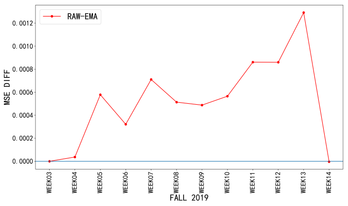
Figure 2 shows the performance of weekly prediction models for test set data. The difference between original data and EMA (RAW-EMA) is plotted in the figure. A value above zero indicates that RAW has a larger error (worse) than EMA on that point. EMA performs equal to or better than raw data in all 12 models. We can then confirm that EMA can smooth the fluctuating time series and better reveal trend information.

Dissimilarity Selection on Real Data

In this subsection, we compare the performance of KLD over mean difference (MDF) and absolute distance (AD) using real-life attendance data.

To confirm the performance of dissimilarity measurements on real-life data, we apply the three methods on attendance data of students from Cohort 2018 in week 8 and week 9 in the Fall 2018 semester. We compare the weekly attendance rate between students whose CGPA (measured after Fall 2018) are in the top 25% quantile (297 students) and last 25% quantile (298 students). Weekly attendance rates in a subpopulation are divided into 5 levels, as is illustrated in Figure 3. Larger inner structure difference is detected in week 9 than in week 8, especially for the lowest attendance category (<0.6).

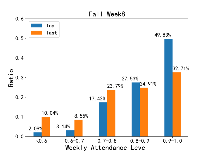
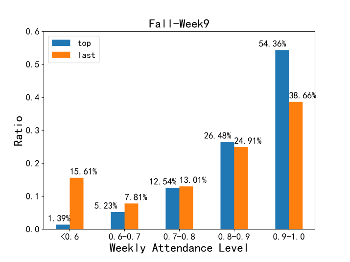
The dissimilarity values between top and last 25% students calculated from the three measurements are shown in Table 3. KLD derives significantly more divergent result for the two weeks (Week 8 and 9), which is consistent with Figure 3. AD cannot detect the divergence order. As KLD could put more emphasis on their most different part, it is more suitable for attendance group comparison.

© 2022 Copyright is held by the author(s). This work is distributed under the Creative Commons Attribution-NonCommercial-NoDerivatives 4.0 International (CC BY-NC-ND 4.0) license.