ABSTRACT
This paper studies the use of Reinforcement Learning (RL) policies for optimizing the sequencing of online learning materials to students. Our approach provides an end to end pipeline for automatically deriving and evaluating robust representations of students’ interactions and policies for content sequencing in online educational settings. We conduct the training and evaluation offline based on a publicly available dataset of diverse student online activities used by tens of thousands of students. We study the influence of the state representations on the performance of the obtained policy and its robustness towards perturbations on the environment dynamics induced by stronger and weaker learners. We show that ‘bigger may not be better’, in that increasing the complexity of the state space does not necessarily lead to better performance, as measured by expected future reward. We describe two methods for offline evaluation of the policy based on importance sampling and Monte Carlo policy evaluation. This work is a first step towards optimizing representations when designing policies for sequencing educational content that can be used in the real world.
1. INTRODUCTION
E-learning platforms have seen a surge in popularity over the last decade [10], spurred on by the increased Internet penetration into developing communities [4]. The target demographic has expanded beyond casual users/students as more organizations adopt e-learning to train their workforce and actively engage them in life-long learning [34].
As online educational settings become ubiquitous, there is a growing need for a personalized sequencing of content/support that can adapt to the individual differences of the student as well as their evolving pedagogical requirement throughout the course progression [28]. Research in cognitive science has long demonstrated the strong correlation between adapted material sequencing and learning outcomes [26]. Static e-learning platforms lack the capacity to respond to a student’s ‘cognitive state’ and therefore perform poorly relative to a human tutor [34].
Reinforcement learning (RL) offer a potential approach for adapting a learning sequence to students [9]. A learning sequence can be optimized based on a numerical reward (for example test marks) by a pedagogical agent that prescribes actions (adaptive feedback or sequencing of content) based on different states (approximated users’ cognitive states).
There are two main challenges to using RL ‘out of the box’ in educational settings. First, how to choose the best representation to model student behavior? On the one hand, increasing the granularity dimension of the state-space allows to capture intricate dynamics in the model such as students’ cognitive states and skills. On the other hand, models with complex state spaces are inherently more difficult to learn and the resulting policy may lack support in the data for parts of the state space. Second, how to evaluate the resulting sequencing policy? Ideally, sequencing policies will be deployed online and evaluated with real learners. This is costly or not technically feasible to carry out in many cases and an imperfect policy may adversely affect students’ learning.
This paper addresses both of these challenges in the context of a new publicly available dataset containing the online interactions of thousands of students [7]. Our approach provides an end to end pipeline for automatically deriving and evaluating robust representations of students’ interactions and policies for content sequencing in online educational settings.
To address the first challenge, we present a new greedy procedure to augment the representation space, by incrementally adding new features and choosing the best performing representations on held out data. Each policy is evaluated using expected cumulative reward. We provide several key insights about the use of RL in Educational contexts. First, that ‘bigger is not always better’, in that more complex state spaces may not always lead to better policy performance. Second, that including a ‘forgetting’ element in the state space, which is known to affect students’ learning, significantly improved performance. Third, that strongly penalizing rewards from unseen state-action pairs in the data, can increase the support of the resulting policy without reducing performance.
To address the second challenge, we use two existing offline policy evaluation methods to reliably estimate the performance of the resulting policy using only the collected data. The first method uses importance sampling to correct for the difference in distributions between the learned policy and the policy that was used to gather the data. The second method simulates the learned policy using Monte Carlo methods. We also introduce a new approach that evaluates the policy with respect to perturbations induced by stronger and weaker learners. We find that perturbing the system dynamics have an adverse affect on performance of the learned policy, specifically in respect to weaker learners; and that increasing the granularity of the state-space makes the policy more robust to perturbations.
This work is a first step towards optimizing representations when designing policies for sequencing educational content that can be used in the real world. Our long term goal is to develop an adaptive RL based pedagogical agent that is able to optimize the sequence of learning materials (questions and lectures) to maximize student performance as measured by the expected ability to answer questions correctly at varying levels of difficulties. This agent will have the capacity to respond in real-time to a student’s current state as they progress through the learning material.
2. RELATED WORK
This paper relates to prior work in student modeling as well as automatically sequencing educational content to students [9]. A common approach in prior work is to integrate learning/cognitive theory into the construction of the student model. This imparts domain knowledge into the workflow and was shown to yield positive results by Doroudi et al. [9]. An example of such approach is the work by Bassen et al. [2]. Their objective was to optimize the sequencing of learning material from different knowledge components (KCs), to ‘maximize learning’. Their reward function is based on the difference between a post-test score (taken by users after completing the course) and a pre-test score (taken before the course). This metric is denoted as the Normalized Learning Gain (NLG). Training the agent with human participants is far too resource intensive. Instead their training is performed on a ‘simulated learner’ based on Bayesian Knowledge Tracing (BKT), a cognitive model that aims to estimate a learner’s mastery of different skills. The learner’s response to a particular question can be simulated based on the mastery of the related skill. The parameters of the BKT were set based on domain knowledge. Segal et al. [28] also utilised a similar cognitive based model, Item Response Theory (IRT) [14] to simulate student responses to questions of different level of difficulty. This is especially relevant since their objective was to sequentially deliver questions of differing levels of difficulty (rather than KCs) to maximize learning gains.
Other approaches forgo the framework of established learning models and instead manually design their simulators further integrating domain expertise. Dorcca et al. [8] employed a probabilistic model to simulate the learning process. Instead of sequencing activities by KCs or difficulties, they sequenced activities based on their associated learning style i.e. visual, verbal etc. Therefore, their simulator was manually designed based on research surrounding these principles. Iglesias et al. [15] utilised an expert derived artificial Markov Decision Process to act as the student model. This entails manually describing the state space, transition probabilities and rewards. Similar to previous student models, this MDP can be used to simulate student responses to train the RL agent.
The works described so far do not utilise historical data (i.e., past interactions in the system and their results) to derive their student model. While integrating expert knowledge can be beneficial, a completely data-free proposition could impart strong biases. In our implementation, we take an alternative approach in using a purely data-driven model. There are existing literature which also do the same. For example, the authors of [30, 32, 5, 27] employed data-driven MDPs as their student model. Different than the handcrafted MDP in Iglesias et al. [15], the transition probabilities and reward functions in these MDPs were obtained from the aggregated statistics observed in the dataset. Data-driven student models in literature were not only limited to data-driven MDPs. For instance, Beck et al. [3] utilised a linear regression model denoted as Population Student Model (PSM). PSM was trained on student trace data from a learning software and could simulate time taken and probability of a correct response.
Data-driven simulators require a quality training corpus that is sufficiently large and varied [30, 16]. In contrast to EdNet (a massive dataset collected over several years which we use in this work), the authors of previous papers were limited to much smaller scale datasets that were collected from a single cohort and could not evaluate their policy at scale. Our work is the first to provide an end to end pipeline from a large scale data source to a robust RL sequencing policy.
3. BACKGROUND
In this section we provide some necessary background in Reinforcement Learning & MDPs and briefly describe our dataset.
3.1 RL and MDPs
A Reinforcement Learning (RL) framework is governed by a Markov Decision Process [31, 17, 6] that is defined by the tuple of , where is the state space, represents all available actions, designates the transition probabilities between states conditioned on an action and denotes the reward function that is conditioned on the state, action and observed next state.
The goal of the agent is to maximize the cumulative reward it accumulates from each state. This cumulative reward is usually discounted by a factor raised to the power of , to represent a lower perceived value for rewards received further in the future. The policy is a mapping of optimal actions to each state in . The discounted cumulative reward is denoted as the ‘return’, and the return from a particular state is associated with a policy and the transition dynamics . The reward function ties the agent’s optimization goal with the modeller’s actual objective. Therefore its design must ensure those two criteria are aligned. The expected reward of a state (or the state value) under a deterministic policy can be defined as
(1)where is the action prescribed by the policy at state , is the reward obtained in state given action , is the initial state and is a discount factor.
Model-based RL requires a model that holds information regarding the environment dynamics i.e. the transition probabilities and reward function . It is a common approach in domains where environment interactions are cost prohibitive [16][18]. The model mimics the behaviour of an environment and allows inferences about how the environment will respond to actions [31]. The real-world performance of the extracted policies are heavily influenced by the quality of the constructed model [16].
3.2 Data Description
EdNet [7] is a massive dataset of student logs from a MOOC learning platform in South Korea, Santa, collected by Riiid! AI Research1. Santa covers a preparation course for the TOEIC (Test of English for International Communication) English proficiency exam. There are a total of 131,441,538 interactions collected from 784,309 students on the e-learning platform. These consist of user records of questions attempted, lectures watched and explanations reviewed, along with other meta information. EdNet logs are presented at 4 levels of hierarchy with higher levels providing higher fidelity logs, such as logs of lectures watched and the explanations reviewed. These are recorded in real time to provide an accurate chronological record of the students’ interaction with the platform. EdNet records detailed actions such as playing/pausing lectures and payment related information.
4. METHODOLOGY
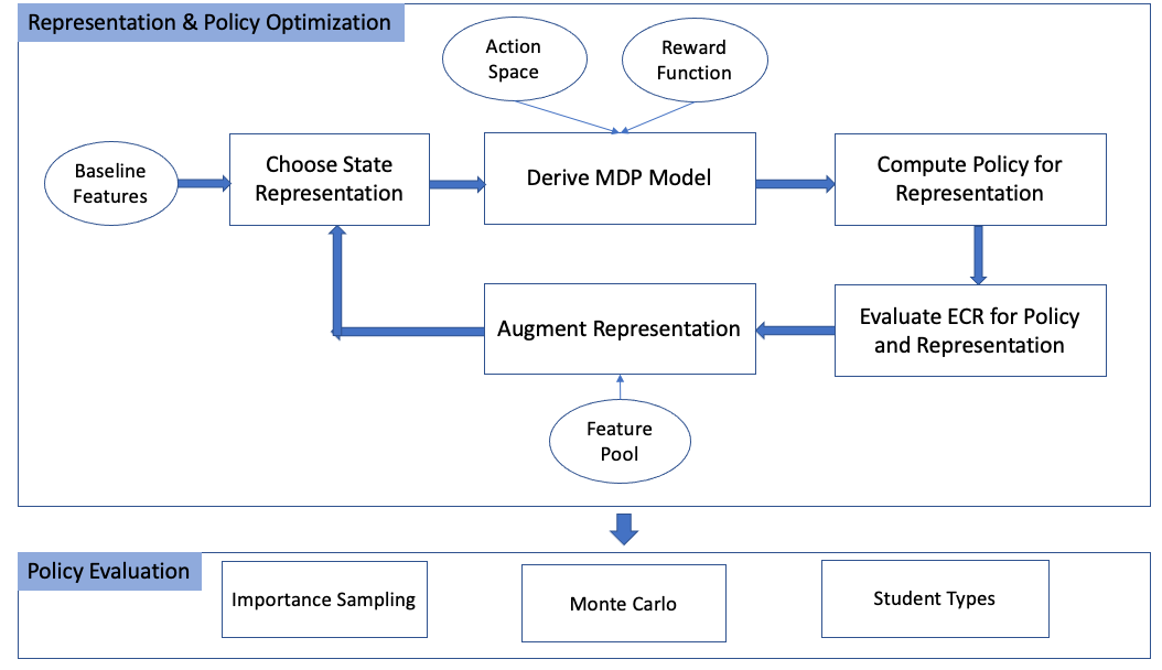
Our approach, called GIFA (Greedy Iterative Feature Augmentation) maps a representation space of students’ activities to an optimal sequencing policy using RL. At each step, a representation-space for the education domain is defined using a set of features. An MDP model is defined over the representation space, and model-based RL is used to extract the optimal policy given the representation space. The policy is subsequently evaluated using the Expected Cumulative Reward metric. This process is iterated, greedily adding new features to the representation and computing the optimal policy given the representation (See top of Figure 1). The resulting representation and policy are verified using two offline policy evaluation processes (importance sampling and Monte Carlo) and the robustness of the policies is analyzed against perturbations corresponding to varying student types (See bottom of Figure 1). We proceed to describing our methodology in more detail.
4.1 State Space Representation
Several studies have shown the significant impact of the representation choice on RL performance, with some arguing it is just as influential as optimization algorithm itself [32, 29]. We design the representation candidates for our model to include features that are derived from the dataset. EdNet provides a total 13,169 questions and 1,021 lectures tagged with 293 types of skills [7]. Each question and lecture is segregated into one unique “part”, with 7 parts in total. Each part was grouped based on some meaningful domain criteria, such as a math topic [2]. EdNet offers a finer grouping of question/lectures according to the ‘skills’ (293 in total) they entail. Both ‘part’ and ‘skills’ grouping represent good candidates for the action space since they group the numerous questions/lectures in a domain meaningful manner. However the question bank is unevenly distributed with respect to the ‘skills’ grouping, which can lead to difficulties in getting equal support (or supporting observations) for each action type from the dataset. Therefore, ‘part’ was chosen on the basis that its 7 unique action space is both computationally feasible and better supported in the data.
A key aspect of modeling student learning is to represent the question difficulty in the state-space [28]. This enables to adapt the level of difficulty of a question to the student’s inferred skill level. Unfortunately EdNet does not directly classify questions/lectures into difficulty levels, meaning that they would need to be inferred from the student logs. A natural way to infer difficulty is to measure the percentage of correct answers submitted for a question and compare it with other questions in the question bank. A distribution over question difficulties can be created and quantiles can be derived to evenly split the questions into discrete levels of difficulty. Utilizing this process we created a difficulty level for each question, with the difficulty levels quantized into 4 levels ranging from 1 (easiest) to 4 (hardest).
To investigate the impact of the representation on performance, we create a feature pool, from which different representations are formed using the greedy iterative augmentation algorithm. The initial feature pool contains features that are widely seen in similar Reinforcement Learning driven Intelligent Tutoring implementations [2, 15, 32, 5]. The state features are longitudinal/temporal in nature so as to represent the users’ behaviour and performance over time. This sets a reasonable minimum requirement for the data gathering process, should this implementation be repeated with other datasets. The initial feature pool, their descriptions, and the associated granularity of their representations (bins), are shown in Table 1. Quantization of features to bins was performed so that a finite model can be formed.
| Feature Pool | Bins | Description |
|---|---|---|
| ”av time” | 4 | The cumulative average of the elapsed time measured at each activity. |
| ”correct so far” | 4 | The ratio of correct responses to the number of activities attempted. |
| ”prev correct” | 3 | A flag to indicate whether the user answered correctly in the previous question + fixed value for lecture. |
| ”expl received” | 4 | Cumulative count of explanations reviewed by the user. |
| ”steps-since-last” | 8 | A count of the number of steps since the current part was last encountered. |
| ”lects consumed” | 4 | A cumulative count of the lectures consumed by a user. |
| ”slow answer” | 2 | A flag to indicate whether the user’s elapsed time for the preceding question was above the average elapsed time for that question. |
| ”steps in part” | 4 | The cumulative count of how many steps a user has spent in the current part. |
| ”avg fam” | 4 | The average part familiarity across all the 7 parts. |
| ”topic fam” | 4 | Captures part familiarity of the previously chosen action (by amount of activities per topic). |
Relative to prior work that limited the feature size to be binary [2, 23, 32] our feature space is considerably larger. With each user covering on average 440 activities during their learning period within this dataset[7], a binary split would lose a lot of information on the evolution of a feature value throughout the course. Our features in contrast have up to 8 bins. This ultimately imposes a necessity for a quality training corpus that can provide sufficient support for each of the many unique combinations within the feature space. This is where the scale of the EdNet dataset provides a distinct advantage relative to previous implementations.
4.2 Deriving the student model
In this section we describe the derivation of an MDP-based student model using a selected set of features. We model the transition probabilities as multinomial distributions derived from state transition counts observed in the dataset as shown in Equation 2. This means that a particular outcome , of enacting action in state has a probability given by the number of times that outcome was observed in the dataset, normalized by the sum of all possible outcomes observed under the same conditions.
(2)Where is the count of observed transitions where enacting action in state leads to next state . This provides the transition probabilities component of the MDP student model for each or the three argument dynamic [31].
In many standard MDP definitions [32, 30, 5], the reward function is also defined in terms of the three argument dynamic i.e. . This assumes a deterministic environment reward with respect to a given . The reward for a student’s response depends on the question difficulty such that correct responses on harder levels indicate stronger performance and attain higher rewards. Inversely, incorrect responses on easier levels attain a larger punishment (negative reward). A symmetrical reward function was designed with rewards for questions ranging from 1 to 4 if answered correctly or -1 to -4 if answered incorrectly. We doubled the penalty of incorrect answers to achieve a normal distribution usually exhibited in student grades [13]. Thus rewards take values . While the level of difficulty is captured by the action in the tuple, the correctness is only captured in the states when ‘prev_correct’ (refer table 1) is included in the representation. Lectures do not have a correct/incorrect responses and so a default reward of ‘0’ is assigned for lecture viewing actions.
The specific dynamic values are of course dependent on the actual state representations. As we continuously augment the representations (see next section), the support for each unique state will inevitably fall due to further division of the observations. Another factor in providing a balanced distribution of support within the transitions, is the variety of actions chosen in each state. This ultimately depends on the action space described earlier and the behaviour policy used to obtain the dataset. A higher fidelity action space will lead to an increase in the size transition space i.e. the unique combinations of . Although unknown in most cases, it is important that the behaviour policy is sufficiently varied in terms of its action choices to ensure a balanced distribution of support. Because of this, a random behaviour policy fits the objective well [30]. Since users in EdNet are allowed to select the ‘part’ and the type of activity they work on [7], we make an assumption that this random criteria is partially fulfilled. The caveat here is that not all users have access to all parts i.e. free users are limited to parts 2 and 5 only.
4.3 Representation Selection
Key to designing a successful model of student behavior depends on deriving information on the student’s cognitive state, which is a latent variable in the model. With more features in the representation, one should expect a better approximation of the students cognitive state and consequently a better equipped pedagogical agent to provide effective sequencing.
We utilise the GIFA approach in obtaining an optimal representation. This involves a search of the feature space and generation of several candidate feature subsets. Each of these subsets is evaluated based on its corresponding policy derived from a standard policy-iteration RL solution. The psuedocode for this process is shown in Algorithm 1. Note the limit on the number of features which can be based on a computational limit or a threshold of minimum support for every unique combination in the feature space.
Set: Optimal feature representation .
while do
for do
Set:
)
end for
Set with highest .
Remove feature from pool
end while
While our search procedure involves exhaustively looping through every remaining feature in the feature pool to form the subsets, one can alternatively employ a different search algorithm such Monte Carlo Tree Search [12] or correlation based feature selection [29] to create more informed subsets that are likely to be better candidates. These techniques would be useful in limiting the number of iterations needed in larger feature pools and are left for future work.
As part of the greedy feature augmentation algorithm above, an evaluation metric for , the computed policy, is required for each representation at every iteration. A common practice used to evaluate a given policy in RL is to use the Expected Cumulative Reward (ECR) metric which is the average of the expected cumulative reward under the policy , across all initial states in the dataset .
Note that in each state representation, the initial state of every user in the EdNet is the same. This is because we lack any prior information of the user before they begin to solve questions. When such information is available, the initial state can capture information from the students pre-test scores and so would vary across the students in the dataset.
5. RESULTS
Round | Rep. | ECR | ECR Diff. (%) |
Rep. Size |
|---|---|---|---|---|
| Base | MDP_B | 238.44 | - | 64 |
| 1 | MDP_1 | 283.63 | 18.95 | 256 |
| 2 | MDP_2 | 387.42 | 36.6 | 2048 |
| 3 | MDP_3 | 392.05 | 1.19 | 4096 |
| 4 | MDP_4 | 396.00 | 1.01 | 16384 |
| 5 | MDP_5 | 396.00 | 0 | 65536 |
| Representation | Features |
|---|---|
| MDP_B | topic_fam, correct_so_far, av_time |
| MDP_1 | topic_fam, correct_so_far, av_time, expl_received |
| MDP_2 | topic_fam, correct_so_far, av_time, expl_received, ssl |
| MDP_3 | topic_fam, correct_so_far, av_time, expl_received, ssl, prev_correct |
| MDP_4 | topic_fam, correct_so_far, av_time, expl_received,ssl, prev_correct, av_fam |
| MDP_5 | topic_fam, correct_so_far, av_time, expl_received, ssl, prev_correct, av_fam, time_in_part |
A summary of the results from the greedy iterative augmentations is provided in Table 2. The feature description for the corresponding MDP representations are given in table 3. The base MDP is denoted as MDP_B. The ‘ECR Diff.’ column shows the percent improvement in ECR relative to the smaller representation preceding it. The ‘Rep. Size’ column illustrates the size of the state feature space. This is dependent on each constituent feature’s bin size, i.e. the number of discrete bins allocated. Note that results presented here are only showing the best performing representation at each round of the feature augmentation.
5.1 ECR Analysis
The largest spike in ECR followed at the second round of augmentations with the addition of the ‘steps-since-last’ (ssl) feature with an increase of 36.6% over the preceding representation. This features measures the number of steps or activities (questions/lectures) consumed since the current part was last encountered. This feature is inferring the ‘forgetting’ element during the learning process and was inspired by the ‘spacing effect’ described in [11].
Early research in instructional sequencing in language learning used models of forgetting to great success [1]. Our findings concur with this, in that by including ‘ssl’ into the feature space, we dramatically increased the policy performance. One could argue that this ECR increase was more influenced by the larger bin allocation to ‘ssl’ (8 relative to 4 for most other features) rather than the actual utility of the domain information it is measuring. However, if that were the case, then we would expect ‘ssl’ to be the first feature added to the base representation. This was not the case since the best performing feature in the first round of augmentations was ‘expl_received’, a 4-size bin feature. Nonetheless, further exploration is needed to further learn the influence of bin sizes on the results.
At the final round of iteration, the performance of representation MDP_5 only equals the performance of preceding representation MDP_4. Though we did not have a specified limit imposed on the number of features, , the performance plateau exhibited at this final round indicated a suitable termination point for the augmentation algorithm. And since MDP_4 produced equal performance to MDP_5 with a smaller representation size, it was chosen to be the optimum representation within this feature pool.
5.2 Correcting for OOD actions
This section describes our technique for handling the uncertainty induced by unseen or out of distribution (OOD) actions in the RL policy. Some of the extracted policies in the GIFA algorithm included state-actions pairs with 0 support from the training data. Such behaviour is deemed unsafe for a computed policy [18, 20] as the resulting reward from such combinations of unsupported state-action pairs is unexpected. Specifically, this situation should not occur under policies derived from tabular methods as explained in section 3. Nonetheless we discovered that some of the larger representations yielded policies with unseen actions. The policy derived from MDP_4 prescribed unseen actions in 10 states. While this was a small fraction of the total state space (around 65,000), unseen actions are an important issue to address because, in the tabular case, any state-action value estimates must be derived only from related experiences [31].
By default, our algorithm prescribes state-action pairs a value of zero if it was never observed. We discovered that the problematic states themselves had very little support in the dataset and were only observed transitioning to themselves, before the episode ends. In the few times the state was visited, a negative or zero reward was produced. Since these states would only transition to themselves, the values of these valid actions were either negative or zero. Hence, from the algorithms perspective, an invalid (unseen) action with a default value of zero, was preferable (or equal) to the observed actions.
To combat this issue, we modified the MDP representations to strongly penalise the rewards from unseen state-action pairs, in the form of a -9999 reward. This discouraged the policy from choosing such actions even if the only valid actions yielded zero or negative returns (The worse case is bounded from below at and is clearly higher than ). With these changes in place, we observe no unseen actions in any of the policies. The performance rank of representations remained constant with the ECR changes almost negligible. This is because the states involved were observed very infrequently and occupied a small probability mass in the transition probabilities. We note that the fix did not have a statistcally significant effect on our results. In the analysis that follows we will utilise the penalised representations. We also note that research by Liu et al. [20] implemented a ‘pessimistic policy iteration’ approach that similarly penalises insufficiently supported state-action tuples (filtered by a threshold).
6. OFFLINE POLICY EVALUATION
Ideally, the outputted policy from the GIFA approach would be evaluated in real time with students who directly interact in the EdNet environment. However, mistakes in the policy can have adverse affects on students’ engagements and learning [21]. The offline policy evaluation (OPE) field has been developed specifically to address this issue, by providing reliable estimates of policy performance using only past collected data [21]. We undertake two different OPE approaches to evaluate the computed optimal policies from the previous sections. Furthermore, we add a 3rd offline evaluation approach which evaluates the robustness of the computed policies to different model perturbations representing several student types.
6.1 Rollouts: Monte Carlo Policy Evaluation
The first OPE approach relies on the family of ‘Direct Methods’ for policy evaluation. These methods focus on regression based techniques to directly estimate the value function of a policy under a given target policy [33]. Most of these methods do not need an estimation of the behaviour policy which was used to collect the dataset. In this method we implement a model-based direct method, Monte Carlo (MC) Policy Evaluation. This involves performing ‘rollouts’ from the initial states using the target policy until episode termination. The observed returns from each state in the rollout are averaged across many rollouts to yield the value function of the state. To ‘rollout’ our policy we would need to interact with the environment. However, as the name ‘model-based’ suggests, a model (in our case, the data-derived MDPs) acting as simulator allows us to perform these rollouts offline.
A key requirement for MC policy evaluation is an episodic environment, one where the episode terminates at a finite step at a ‘terminating state’ [31]. Although the user episodes in EdNet are finite, our data-derived MDPs are continuing i.e. without a terminating state. While a default terminating state could have easily been created for this purpose, it is unclear as to which ‘action’ would transition the final observed state to this terminating state and what ‘reward’ it would receive in the process. The choice of reward, could inadvertently impact the decisions made by the policy at the earlier states. Hence our MDPs were designed to be continuing to avoid this ambiguity.
This poses a problem with MC policy evaluation since the returns are only calculated when the episode ends. A potential workaround was to manually terminate the episode at a fixed length of rollout and calculate the returns from there. We chose a rollout length of 1000 steps and show that because of the discounting, any reward, , received past this step, will have a negligible influence on the return of the initial state i.e. . Hence this rollout length provides a good approximation of the long term return, since any future actions will have minimal influence on the value of the initial state, i.e. the only state value of concern in our analysis. However, this assumption will only work with the ‘first-visit’ variant of MC policy evaluation (equation 3), where only the returns of a state when it was first encountered in the episode are considered and averaged across the rollouts [31]. This is opposed to the ‘every-visit’ variant which considers all the returns from a state every time it is visited in the episode. A fixed rollout length will not be suitable in the latter variant, since the initial state could be encountered more than once during the rollout. For example, if was encountered again at the 500th time step, then its return estimate for the second visit is based only on the remaining 500 future steps. Implementing the first-visit variant ensures that all estimates are derived from observations spanning 1000 time steps ahead.
(3)
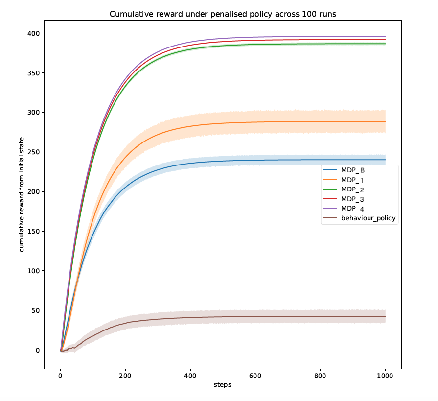
We now evaluate the policies under the MC Policy Evaluation method. A curve is plotted for the returns (cumulative rewards) from the initial state as the rollout progresses until the 1000th step for a total of 100 rollouts. The 95% confidence intervals are plotted around the mean value of the rollouts. This analysis is shown in figure 2. As with the ECR, we can see that the improvements start to diminish significantly after the second round of augmentations. The performance of the estimated stochastic behaviour policy under this simulation (the policy that is directly induced from the data) is illustrated as a baseline. From this comparison, we see much better student performance under the RL policies than the baseline, signalling that the adaptive behaviour of the policy under RL framework is superior than the strategies used in the behaviour policy. We can also conclude that the larger representations exhibit better performance, potentially owing to a better approximation of the cognitive state as hypothesized.
6.2 Importance Sampling Policy Evaluation
The second OPE approach used relies on Importance Sampling. Importance sampling (IS) is a range of methods that in general estimate the expected values under one distributions given samples from another [31]. A wide range of RL literature have adopted this method as a way of evaluating a target policy (the policies derived from the RL algorithms) given samples derived from the behaviour policy (the policy used to gather the data) [16]. In this work we use the Weighted IS (WIS) metric presented in equation 4.
(4)
In this equation, represents the number of users in the dataset and is the trajectory length observed for user .
A key feature in the formula is the importance sampling ratio , which considers the differences in action probabilities between the target policy and the behaviour policy . The product of the individual ratios across quantifies whether a given sequence is more (or less) likely under than and therefore weights the returns accordingly. Averaging this across the entire dataset has the effect of adjusting the expected return sampled from the distribution generated by to estimate the expected return sampled from .
A well documented problem with IS estimators is the high variance induced by the importance sampling ratio due to: 1) a large difference between the two policies or 2) a long horizon length for the trajectories [33]. WIS reduces this variance by utilizing a weighted average instead of the simple average in standard Importance Sampling metric [31]. This method relies on the available knowledge of the behaviour policy. Since we do not have explicit information on this, must be estimated from the dataset, as shown in equation 5.
| Rep. | WIS |
|---|---|
| MDP_B | -4.146 |
| MDP_1 | -0.940 |
| MDP_2 | -4.382 |
| MDP_3 | 4.319 |
| MDP_4 | 4.910 |
The results of the WIS metric for the different representations are shown in table 4. We see that the 3 smaller representations yield negative values, indicting expected average failure in solving questions when utilizing these representations. For larger MDP representations, we can observe better performance, with MDP_4 demonstrating the best estimated performance.
6.3 Evaluating Model Robustness for Different Student Types
The optimal policy computed in the previous section relies on the average rewards and transition probabilities estimated from available data. In practice, these parameters are noisy and may change in different situations and during the execution of a policy [19]. As such, the performance of the computed policy may deteriorate significantly with changes in the environment dynamics [22]. In our case, with the MDP representing students acting in an educational system, this uncertainty represents the challenge of how to model parameters change for different student types and how do these changes influence the outcome of the computed policies. To model this uncertainty, we use a simplified robust MDP framework [25] where the uncertainly in model parameters is tied to specific student types. Specifically, we test the robustness of the computed policies under perturbations of the environment dynamics which are tied to two different student types. These perturbations are domain informed and are designed to correspond to ‘stronger’ and ‘weaker’ students types.
2: for do
3:
Where
4: end for
5: Adjust relative to others within the pair:
6: Set perturbed transition probabilities
7: for do
8:
9: end for
10:
11: Return:
| Feature to Perturb | Strong | Weak |
|---|---|---|
| Topic_fam | ||
| Correct_so_far | ||
| Avg_time |
We now describe the perturbation process and analysis. We define a set of domain informed filters for each perturbed feature. In our implementation we perturb three base features that were common in all representations i.e. ‘Topic_fam’, ‘Correct_so_far’ and ‘Avg_time’. The domain rules for the two separate perturbations ‘Strong’ and ‘Weak’ are defined in table 5. Specifically, in these perturbations we boost the topic familiarity and correctness and reduce the cumulative elapsed time for the ‘Strong’ student type and we reduce correctness and increase the cumulative elapsed time for the ‘Weak’ student type. For example, for the feature ‘Correct_so_far’ and the ‘Strong’ user case, we set the filter to capture transitions where the next state registers a greater or equal value relative to the current state . When this filter is inputted in algorithm 2, the transitions that satisfy this filter will be boosted by the constant . This ultimately has the effect of increasing the probability mass of this transition, perturbing the original MDP to make such transitions more likely.
Algorithm 2 introduces the perturbation process. In lines 2 to 4 we compute the transition probability deltas that are required for every transition which satisfies one or more perturbation filter. This is done for all state transitions in the MDP. In line 5 we create transition deltas for all transitions, accounting for the deltas introduced by the perturbed transitions. In lines 6 to 9 we apply the transition deltas to the transition probabilities, and finally in line 10 we normalize the transition probabilities following the changes made.
The results of two separate perturbations are measured by performing a policy evaluation algorithm with the original policy but under the perturbed MDPs (Strong & Weak) as the simulators.
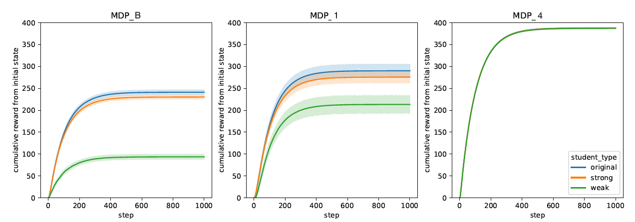
Figure 3 shows the results of this analysis for the different representations. Notice that in all the representations, the original non-perturbed MDP always yielded the best performance (non-visible for MDP_4 as the student type lines overlap). This is expected, since the original policy was derived to perform optimally on the original MDP. However, as the representation size increases, the effects of the perturbations becomes less pronounced, almost becoming negligible past MDP_1. To determine if the larger representation would be affected with more features perturbed, we conducted another round of perturbations, this time only on MDP_4 and with all of its features (barring ‘ssl’) perturbed. The results show that the performance of the policy was not affected by the extended perturbations. This means that the MDP_4 is more robust towards deviations from the expected dynamics derived from the data. Hence, we have increased confidence that such policies would be robust in the real-world setting, maintaining their performance for students that exhibit different learning characteristics than those averaged over the observations in the EdNet dataset.
Taking the three offline evaluation results in combination we conclude that MDP_4 demonstrated the best performance across representations and perturbations.
7. DOMAIN RELATED INSIGHTS
By analyzing the state values and the policies derived from the RL algorithms, we can discover interesting insights in the way the policy behaves with respect to different learners. We demonstrate this approach on the simpler MDP_B which is based on the 3 features: topic familiarity, correct so far and average time. In figure 4, we plot the derived state values against the av_time and correct_so_far features in MDP_B. Based on our reward design, the state values indicates the future user performance. The expected future performance of the policy is much higher when the student has a high correct_so_far answer ratio. However, the relationship between the average time and state values is more complex. At higher values of ‘correct_so_far’, a higher ‘av_time’ entails a larger state value, but when ‘correct_so_far’ is low, the opposite is true and in such a case lower values of ‘av_time’ entails a larger state value. This means that for students with lower success so far, faster average time is indicative of higher future success. We hypothesize that this is due to the policy’s inability to significantly assist students which are consistently unsuccessful in solving questions and which are also taking relatively long time to dwell on each and every question. We note that even if the policies themselves are not used, findings like this can inform us of useful features and their relationships in predicting future user performance following informed interventions. Such findings can also inform us on the limits of automated approaches, and on the need for additional tailored support for struggling students, e.g. by supplying personalized human assistance where automated approaches are expected to demonstrate low effectiveness.

Analyzing the action choices in the policies, we discover that the RL algorithms tend to put preference on level 4 actions (harder questions). Indeed these do yield the highest reward and the lowest punishment in our reward design. One possible extension is to investigate how a change in the reward function design would impact the policy preferences. Again, even if the computed policies are not deployed in the field, such analysis can be useful as a technique in letting the data guide pedagogical strategies, for example by connecting pedagogically justified rewards to sequencing policies that maximize such a reward given the available data.
8. CONCLUSIONS AND FUTURE WORK
In this paper we approached the challenge of designing an adaptive RL based policy for optimizing the sequencing of learning materials to maximize learning. Human tutors usually outperform their computer counterparts, in that they are able to adapt to certain cues exhibited by the student during learning [34]. Training an RL policy with actual users is far too resource intensive. Therefore, we simultaneously tackle the problem of training and evaluating an RL algorithm offline based only on pre-collected data. A purely data-driven student model was created for this purpose. We hypothesized that a complex model is required to capture the intricacies of human learning. To investigate this theory, a large dataset, EdNet, was necessary to provide sufficient support for the models.
Our student model was constructed in the form of a data-derived MDP, with the transition and reward dynamics estimated from the observations in the data. The raw logs were transformed into domain inspired features. By using the MDPs we then trained our agents with the model-based Policy Iteration algorithm. To determine whether a more complex model yields better tutoring, we employed a greedy iterative augmentation procedure. The ECR metric guided how we chose our features and demonstrated the positive relationship between representation complexity and policy performance. In our analyses we discovered issues with Out of Distribution actions in the policies and presented a solution in the form of penalising rewards. We further evaluated our policies using the Monte Carlo and Importance Sampling Policy Evaluation algorithms and tested the policies robustness against domain informed perturbations of the dynamics. We show that the larger representation are less impacted by the perturbations and therefore can provide a more equal learning experience for stronger or weaker students.
Several limitations are acknowledged which consequently open up further investigations. The influence of the bin-size on feature preference in the representations was discussed briefly but lacked conclusive evidence to rule out entirely. This work is necessary to ensure that the features are selected based only on the utility of the domain information they capture. From our model-based policy analyses we also discovered out-of-distribution actions in the policy space. Though we managed to remedy the problems for completely unseen actions through strong penalisation, the next course of action is to also penalise low supported actions/states variably according to their uncertainty as was explored by [20, 35]. We would also like to compare our approach to other feature selection and augmentation algorithms, such as genetic based metaheuristics [24]. Finally, the inferred policies should be evaluated in the real world in a controlled study.
9. ACKNOWLEDGEMENTS
This work was supported in part by the European Union Horizon 2020 WeNet research and innovation program under grant agreement No 823783
10. REFERENCES
- R. C. Atkinson. Optimizing the learning of a second-language vocabulary. Journal of experimental psychology, 96(1):124, 1972.
- J. Bassen, B. Balaji, M. Schaarschmidt, C. Thille, J. Painter, D. Zimmaro, A. Games, E. Fast, and J. C. Mitchell. Reinforcement learning for the adaptive scheduling of educational activities. In Proceedings of the 2020 CHI Conference on Human Factors in Computing Systems, pages 1–12, 2020.
- J. Beck, B. P. Woolf, and C. R. Beal. Advisor: A machine learning architecture for intelligent tutor construction. AAAI/IAAI, 2000(552-557):1–2, 2000.
- J. Capper. E-learning growth and promise for the developing world. TechKnowLogia, 2(2):7–10, 2001.
- M. Chi, K. VanLehn, and D. Litman. Do micro-level tutorial decisions matter: Applying reinforcement learning to induce pedagogical tutorial tactics. In International conference on intelligent tutoring systems, pages 224–234. Springer, 2010.
- M. Chi, K. VanLehn, D. Litman, and P. Jordan. Inducing effective pedagogical strategies using learning context features. In International conference on user modeling, adaptation, and personalization, pages 147–158. Springer, 2010.
- Y. Choi, Y. Lee, D. Shin, J. Cho, S. Park, S. Lee, J. Baek, C. Bae, B. Kim, and J. Heo. Ednet: A large-scale hierarchical dataset in education. In International Conference on Artificial Intelligence in Education, pages 69–73. Springer, 2020.
- F. A. Dorça, L. V. Lima, M. A. Fernandes, and C. R. Lopes. Comparing strategies for modeling students learning styles through reinforcement learning in adaptive and intelligent educational systems: An experimental analysis. Expert Systems with Applications, 40(6):2092–2101, 2013.
- S. Doroudi, V. Aleven, and E. Brunskill. Where’s the reward? International Journal of Artificial Intelligence in Education, 29(4):568–620, 2019.
- E. Duffin. E-learning and digital education-statistics & facts. Retrieved December, 22:2019, 2019.
- H. Ebbinghaus. Über das gedächtnis: untersuchungen zur experimentellen psychologie. Duncker & Humblot, 1885.
- R. Gaudel and M. Sebag. Feature selection as a one-player game. In International Conference on Machine Learning, pages 359–366, 2010.
- T. Grosges and D. Barchiesi. European credit transfer and accumulation system: An alternative way to calculate the ects grades. Higher Education in Europe, 32(2-3):213–227, 2007.
- R. K. Hambleton, R. J. Shavelson, N. M. Webb, H. Swaminathan, and H. J. Rogers. Fundamentals of item response theory, volume 2. Sage, 1991.
- A. Iglesias, P. Martínez, R. Aler, and F. Fernández. Reinforcement learning of pedagogical policies in adaptive and intelligent educational systems. Knowledge-Based Systems, 22(4):266–270, 2009.
- S. Ju, S. Shen, H. Azizsoltani, T. Barnes, and M. Chi. Importance sampling to identify empirically valid policies and their critical decisions. In EDM (Workshops), pages 69–78, 2019.
- H. Le, C. Voloshin, and Y. Yue. Batch policy learning under constraints. In International Conference on Machine Learning, pages 3703–3712. PMLR, 2019.
- S. Levine, A. Kumar, G. Tucker, and J. Fu. Offline reinforcement learning: Tutorial, review, and perspectives on open problems. arXiv preprint arXiv:2005.01643, 2020.
- S. H. Lim, H. Xu, and S. Mannor. Reinforcement learning in robust markov decision processes. Advances in Neural Information Processing Systems, 26, 2013.
- Y. Liu, A. Swaminathan, A. Agarwal, and E. Brunskill. Provably good batch off-policy reinforcement learning without great exploration. Advances in Neural Information Processing Systems, 33:1264–1274, 2020.
- T. Mandel, Y.-E. Liu, S. Levine, E. Brunskill, and Z. Popovic. Offline policy evaluation across representations with applications to educational games. In AAMAS, volume 1077, 2014.
- S. Mannor, D. Simester, P. Sun, and J. N. Tsitsiklis. Bias and variance approximation in value function estimates. Management Science, 53(2):308–322, 2007.
- Y. Mao. One minute is enough: Early prediction of student success and event-level difficulty during novice programming tasks. In In: Proceedings of the 12th International Conference on Educational Data Mining (EDM 2019), 2019.
- S. Mirjalili. Genetic algorithm. In Evolutionary algorithms and neural networks, pages 43–55. Springer, 2019.
- A. Nilim and L. El Ghaoui. Robust control of markov decision processes with uncertain transition matrices. Operations Research, 53(5):780–798, 2005.
- F. E. Ritter, J. Nerb, E. Lehtinen, and T. M. O’Shea. In order to learn: How the sequence of topics influences learning. Oxford University Press, 2007.
- J. Rowe, B. Pokorny, B. Goldberg, B. Mott, and J. Lester. Toward simulated students for reinforcement learning-driven tutorial planning in gift. In Proceedings of R. Sottilare (Ed.) 5th Annual GIFT Users Symposium. Orlando, FL, 2017.
- A. Segal, Y. B. David, J. J. Williams, K. Gal, and Y. Shalom. Combining difficulty ranking with multi-armed bandits to sequence educational content. In International conference on artificial intelligence in education, pages 317–321. Springer, 2018.
- S. Shen and M. Chi. Aim low: Correlation-based feature selection for model-based reinforcement learning. International Educational Data Mining Society, 2016.
- S. Shen and M. Chi. Reinforcement learning: the sooner the better, or the later the better? In Proceedings of the 2016 conference on user modeling adaptation and personalization, pages 37–44, 2016.
- R. S. Sutton and A. G. Barto. Reinforcement learning: An introduction. MIT press, 2018.
- J. R. Tetreault and D. J. Litman. A reinforcement learning approach to evaluating state representations in spoken dialogue systems. Speech Communication, 50(8-9):683–696, 2008.
- C. Voloshin, H. M. Le, N. Jiang, and Y. Yue. Empirical study of off-policy policy evaluation for reinforcement learning. arXiv preprint arXiv:1911.06854, 2019.
- B. P. Woolf. Building intelligent interactive tutors: Student-centered strategies for revolutionizing e-learning. Morgan Kaufmann, 2010.
- T. Yu, G. Thomas, L. Yu, S. Ermon, J. Zou, S. Levine, C. Finn, and T. Ma. Mopo: Model-based offline policy optimization. arXiv preprint arXiv:2005.13239, 2020.
1https://www.riiid.co/
© 2022 Copyright is held by the author(s). This work is distributed under the Creative Commons Attribution-NonCommercial-NoDerivatives 4.0 International (CC BY-NC-ND 4.0) license.