ABSTRACT
Student grade prediction is a popular task for learning analytics, given grades are the traditional form of student performance. However, no matter the learning environment, student background, or domain content, there are things in common across most experiences in learning. In most previous machine learning models, previous grades are considered the strongest prognosis of future performance. Few works consider the breadth of instructor features, despite the evidence that a great instructor could change the course of a student’s future. We strive to determine the true impact of an instructor by analyzing student data from an undergraduate program and measuring the importance of instructor-related features in comparison with other feature types that may affect state-of-the-art student grade prediction models. We show that adding extensive instructor-related features improves grade prediction, when using the best supervised learning classifier and regressor.
Keywords
1. INTRODUCTION
Student performance prediction is a useful service for multiple educational stakeholders in a university and other educational contexts. For example, it is a frequent feature in learning analytics software, like in early-warning systems [6], curriculum personalization [5], cultivating student study skills [13], characterizing course difficulty [31], and can be incorporated into Intelligent Tutoring Systems [22], Massively Open Online Courses [26], and Learning Management Systems [17]. It makes sense that a student would want to use their predicted grade in future courses for short-term course planning, or if an instructor or advisor would want to predict the grades of their students as an early indication of which students are likely to need more assistance.
Intuitively, it would appear that student history would be sufficient to predict future grades. However, in a classroom environment,the student and their past grades are not the only factors that dictate the student’s performance. The specific course for which the grade is being predicted and the particular instructor can also affect the outcome of the student’s efforts. It is common knowledge that students have varying strengths and weaknesses that interact with courses and their materials. This is reflected in machine learning (ML) models that attempt to carry out student grade prediction by including course-based features. Furthermore, the content of the course and the student’s ability to retain the information and skills they learned can also have an impact on student performance (e.g. [27]). Similarly, it is also known that instructors can have a monumental impact on students. For example, good teachers can improve standardized testing scores in reading and math [20]. When considering a teacher’s motivation level, there is a direct link to students’ academic achievement [4]. Furthermore, it is a common anecdote for someone to be able to point to a teacher that had greatly affected who they became later in life, usually by reinforcing positive traits or shielding from negative influences (e.g. [9]). Yet, an instructor’s impact on a student’s performance has not been fully explored, quantitatively and in ML models.
In this paper we take a first step to characterize the feature space that can describe the instructor effect on student grade prediction. We experiment with several ML algorithms, using a dataset with thousands of student data records from a large, public university, and show that adding extensive instructor-related features improves grade prediction. Our evaluation shows that GradientBoost is the best supervised learning classifier and regressor, and we will use it to compare instructor-based features with other feature types.
2. PREVIOUS WORK
Student performance prediction is a popular research subject, given its varied applications and approaches. Some works have approached the problem of binary classification of student performance (e.g., predicting pass/fail), to focus educators’ attention to the needy students. However, our focus is on overall prediction of the Grade Point Average (GPA) of the final grade in a course, along with a corresponding 5-class breakdown of the grade1, to explore the possible effect that instructor features have over a course’s final grade. Many works also attempted to train models that predicted multi-class classification (e.g., categorical/letter grading) or regression (e.g., percentage) [1], but with no attempt to include instructor characteristics.
Recent published work in grade prediction has focused on experimenting with different ML models, using features such as student characteristics, domain content, or other course characteristics. Morsy and Karypis [19] focused on assigning knowledge component vectors for each course, paired with a student’s performance in those courses, to inform a regression model, and attained up to 90% accuracy for some predictions with leeway up to 2 half-grades away2. Polyzou and Karypis [25] employed Matrix Factorization, previously found in recommendation systems, and focused on historical student grades as the primary feature category, achieving an average error between 2 to 3 half grades. Widjaja et al. [34] combined a Matrix Factorization model, Factorization Machines (FM), with a Long Short-Term Memory neural network, using multiple course and student features, achieving an error between 1 to 2 half grades. None of these works included instructor-based features. For comparison, we will use an FM [29] model as one of our baselines.
Most research to date in this area focuses on past student performance, student-based features, and more recently on course-based features, like in the examples given above. Polyzou [24] went further in an attempt to enumerate student grade and course-based features, but applied the models only to predicting several binary classifications (e.g. will the student fail the course?). They found that for some classification tasks, some feature types improved the performance, while in other classification tasks, they made things worse.
Given that our focus is to add instructor features, we examined works that included them. Ren et al. [28] used only an instructor’s ID when training a neural collaborative filtering model and achieved an error within two half grades. Zhang et al. [35] had a feature list that included 4 instructor-based features (that were grouped with course-based features), namely “teacher’s seniority, teacher’s age, teacher’s title, [and] teacher’s nation.” They applied a variation on a Convolutional Neural Network, achieving an F1-score of 0.805 for a 5-grade classification task. Hu et al. [14] included three instructor features in their datasets, namely instructor’s rank, tenure status, and average GPA over all of the courses they taught in the dataset; they achieved an average error up to 1 grade level difference with regression. Sweeney et al. [32] used 4 instructor features, classification, rank, tenure status, and a bias term introduced in their model, features which focused on their official positions rather than experience, and achieved an error range of two half grades. Each of these works haphazardly included a few instructor features. Only Sweeney et al. analyzed the instructor features’ effects on the performance of their chosen models, and found that the instructor’s bias feature was the third-most important feature, yet was only one-third as important as the student’s bias feature. Our work makes headway in instructor-based features, and examines the number and importance of such features in more detail.
3. DATASET
3.1 Program Curriculum
The dataset is taken from a computer science (CS) four-year, undergraduate degree program at the main campus of a large American public university. This university has four independent satellite campuses that may offer similar courses, but do not offer the same curriculum. However, it is common for students to transfer from satellite campuses to the main campus and enroll in the CS degree, and some courses students took at the satellite campuses can be transferred into the main campus’ CS program with approval from the main campus undergraduate program director.
Courses in the program are split into three categories: mandatory, electives, and a capstone. There are 8 mandatory courses that all students who intend to graduate with a CS degree must take (unless students will enter with Advanced Placement/International Baccalaureate CS credit or transfer courses from other campuses). For electives, students pick at least 5 upper-level CS courses that pertain to their interests and strengths. Each course may or may not contain prerequisites, and if they do, they tend to be other CS courses. Some mandatory courses have co-requisites, meaning certain courses may be taken at the same time. Students must pass each course with a grade of “C” or higher; if a student does not reach this threshold, they are given the opportunity to retake the course up to two additional times. The last grade that the student received for a course, regardless if it is higher or lower than any previous attempt, is the final grade recorded for the course. The capstone is a project-oriented course as a culmination of the CS curriculum, but not relevant to this research.
Instructors are given flexibility in how they wish to teach their course, as long as they follow the generalized syllabus that is agreed upon by the area faculty for that course. The syllabus contains a list of topics that instructors are expected to cover, but does not prescribe the depth that the instructor must reach for each topic. Should instructors believe there are additional important topics not covered by the generalized syllabus, they are also free to add them into their course. A specific order is similarly not imposed by the generalized syllabus, but topics tend to build on each other naturally, common in STEM fields (e.g. [15]), which imposes a soft ordering. However, due to individual preferences on how to present concepts to students, instructors have the freedom to conduct their courses differently. Given different degrees are offered on satellite campuses, we expect that in the same course, satellite instructors will present their concepts differently from instructors in the main campus.
The main campus CS degree program also is involved in a college-in-high-school (CHS) program, where the CHS program director and a faculty liaison provide materials to high school teachers, and if the student earns a passing grade given by the high school teacher, they qualify for college credit, as if the student took the course at the university. The material high school teachers receive is more structured than the generalized syllabus that instructors for undergraduate students receive, and the university provides training for those teachers to ensure the material that is taught is at the same level of rigor as what is expected for the undergraduate course. The high school teachers assign the final grade, which are recorded in the official university transcripts.
3.2 Summary Statistics
Upper bound due to 3,786 courses missing instructor data.
Upper bound due to 408 CS CHS courses missing instructor data.
Transcripts of 3,646 students, all of whom enrolled in at least one of the first two computer science major mandatory courses (since those two can be taken in any order and have no prerequisites) were retrieved from the university registrar. Records spanned between August, 2006 and December, 2019, for a total of 186,316 grade records. Not all students have completed the degree program, but the university does not have an official denotation for when students have decided they no longer wish to pursue their studies at the university or are taking a break from their studies.
3.3 Data Cleaning
To retain consistency, students enrolled in the computer engineering (CE) program, which for a time took many of the same mandatory courses of the CS program, but with a different passing grade requirement, were removed from the set, leaving 3,122 students. We further cleaned the dataset by removing all non-CS courses and non-letter grades (e.g. “Withdraw”, “Satisfactory”, etc.), leaving 28,150 “fully-cleaned” grade records. Basic statistics can be found in Table 1.
4. METHODOLOGY
Our goal is to generate a supervised ML model that can predict a student’s grade for a target CS course in a given semester of their undergraduate career, and use that model to run a comparison between the different feature types (i.e., to figure out which feature types contribute the most to the best prediction), which will include instructor features.
4.1 Features
We include four types of features in our models: Student Characteristics, Student Grade History, Course Characteristics, and Instructor Characteristics, as detailed below. There are 571 features altogether. The first feature that we include with any model we will train is the target course number, to indicate which course the training grade label came from.
4.1.1 Student Characteristics
Student Characteristics are features that describe the student themselves that are not directly related to their courses. We include a student’s ethnic group, gender, math and verbal SAT scores, ACT scores3, high school GPA, whether they are the first in their family to attend college, and whether they are an in-state or out-of-state student. Furthermore, with the anecdotal knowledge that instructors have particular jargon, preferences, and quirks, we add a feature indicating if the student has ever encountered the same instructor for the target course, or if the instructor was the same for the target course’s prerequisite, in the belief that a student who encounters the same instructor again has a better understanding of how to satisfy the instructor’s requirements. This provides a total of 9 features.
Demographic breakdown of the students in the dataset can be found in Table 2.
4.1.2 Student Grade History
Student Grade History features are a simple enumeration of all CS courses a student has taken in their undergraduate career. Each course is represented by a pair of features, the grade they received as a GPA value (e.g., 4.0 instead of A), and the semester number they took the course relative to the first CS course they took, which includes the summer term. As an example, assume a student took their first ever CS course, CS 101, in the spring term and received a B, and took CS 102 in the fall term of the next school year and received a A; the resulting grade and semester pairs for CS 101 and CS 102 would be and , respectively. We use relative semester value given that students have other general education requirements to fulfill not related to the major, and thus can choose to delay taking CS courses, or take the initial CS courses more leisurely. This provides a total of 218 features. Note that each feature will be considered independently when training the models.
The grading scale, GPA-equivalent, and distribution of grade records can be found in Table 3.
4.1.3 Course Characteristics
Course Characteristics describe the courses. We generate these characteristics for the target course, which will be the direct context that the model can use in the grade prediction task. We include the target course’s semester relative to the student’s first semester taking a CS course and maximum enrollment size. We also compile the history of grades for the target course before the semester the student completed the course by providing the parameters that describe their fitted distributions over the GPA-equivalent conversion. We provide the Weibull distribution, which can be described over three parameters: location, shape, and scale, aside from the normal distribution’s mean and standard deviation. Lastly, we derived a feature to denote whether the target class started in the morning (AM) or afternoon and evening (PM). For completeness, we also provide the maximum enrollment size for all courses the student has taken. This provides a total of 117 features.
4.1.4 Instructor Characteristics
Instructor Characteristics describe a target course’s instructor, and were chosen here as an attempt to reflect the instructor’s tendencies and experience, which, under our hypothesis, may have an effect on student performance. We generated the cumulative number of students taught by that instructor in any course to characterize the instructor’s experience. In addition, we include the instructor’s official rank at the time of the target course. In understanding an instructor’s grading behavior, we consider the instructor’s past history of assigning grades, in an attempt to capture how “demanding” the instructor is, by including features that describe the distribution of the instructor’s given grades. We generated the Weibull distribution parameters, location, shape, and scale, along with the mean and standard deviation, for the collection of grades that the instructor has assigned for the target course, for all courses they have ever taught, and for grades they have given for only morning or evening classes. For completeness, we include the instructor’s ID as a base feature for every course the student has taken (or null if the student has not taken the course at the time of the target semester), representing the history of instructors that the student has encountered. This provides a total of 226 features.
Relating to instructor’s official rank, the CS department under study has several official teaching positions, namely “Teaching Fellow,” “Part-Time Instructor,” “Lecturer,” “Senior Lecturer,” “Visiting Lecturer,” “Visiting Professor,” “Assistant Professor,” “Associate Professor,” and “Full Professor.” We opted to merge “Teaching Fellow” with “Part-Time Instructor,” given their duties are exactly the same, but the former corresponds with PhD students. Each instructor’s rank was consistent with the position they held at the beginning of the semester that they taught a course. In addition, we included another category, “High School Teacher,” to indicate teachers who taught through the college-in-high-school program, given students who are enrolled in the program may have a CHS course (or several) on record. Finally, we include a “Satellite Instructor” title, given the courses taught at the satellite campuses are different, despite the true title that those instructors have.
4.2 Comparison Metrics
We compare the models using weighted average F1-score (Weighted F1) for classification, as well as mean absolute error (MAE) and root mean square error (RMSE) for regression. We also conduct cross-metric comparisons for completeness. For computing MAE and RMSE for each classifier, we converted the predicted letter grade directly into their corresponding GPA value. For computing Weighted F1 for each regressor, we took the predicted value output, which represents an expected GPA, converted it to the closest letter grade, and dropped the plus or minus, where applicable. Conversions between GPA values and letter grades can be found in Table 3.
The F1-score formula is defined as
where TP is the true-positive rate, FP is the false-positive rate, and FN is the false-negative rate. For multiclass classification, weighted average F1-score formula is defined as
where is the F1-score for class , and is the number of data points that are part of class . This metric gives more weight towards correctly predicting larger-sized classes.
The MAE is defined by the following formula
where is the value predicted by the algorithm, is the true value, and is the number of data points. MAE can be preferred for grade prediction because the absolute distance can translate directly into GPA values without additional penalty for significant wrong predictions.
The RMSE is defined by the following formula
where , , and have the same definitions as those in the MAE formula. As opposed to MAE, RMSE penalizes large errors, which can be useful in spotting cases where excellent grades are predicted as failing grades, and vice versa.
Note that higher values of Weighted F1 mean the model is better, while for MAE and RMSE, lower values mean that the model is better.
4.3 Data Preparation and Model Selection
Recall that the task is to predict the grade of a student for a target course. Towards that aim, we first clean the dataset as described in Section 3.3, and then compile the features for each student, ensuring that the feature vector is consistent with the known information at the time they would be taking the course, so that future information cannot inform past courses. For example, if the student is taking CS 102 in the third semester, then only grades from before the third semester will be part of the input. Note that, for the purposes of training the algorithms, we ignore prediction for CS courses offered for non-majors, given that CS students are unlikely to be taking those courses, especially after they have already started taking the mandatory courses. As a result, the total dataset transformed into 25,354 rows, an average of 7.7 transcript moments (or courses and grades) per student considered. The dataset was randomly split 80-20 for training and testing, respectively.
We decide to compare several classifiers and regressors, as described below. We use implementations by Scikit-learn [23], unless otherwise noted. For the classification task, we only require the models to predict from the five letter grades (i.e. {A,B,C,D,F}, where is dropped). For the regression task, we train the models to predict GPA values using the university’s scale (found in Table 3).
We train five different classifiers: majority classification (Majority) as a baseline, decision tree model (DT), -neighbors model (, 2Neigh), AdaBoost classifier (AdaClass), and GradientBoost classifier (GradClass). To reduce variability, we utilize five-fold training; we tested typical cross-validation, “soft” voting, and “hard” voting [21]. We explain the first two here for completeness, and we report soft voting because it yielded the best results. In typical 5-fold cross-validation (we assume 5 folds in this paper), five mutually-exclusive and equally large portions of the training set are generated, the classifier is trained on four folds of the data and validated on the fifth, generating a model instance. This procedure is repeated five times, generating 5 different classifier model instances trained on different subsets of the data. We then select the instance with the best performance, and use that model to label new input. In five-fold soft voting, rather than selecting one instance, we average across all instances, and the class with the highest average is the label assigned to the input.
Due to the imbalance of the classes (see Table 3 for a breakdown), we attempted class-balancing via upsampling and downsampling (e.g. SMOTE [8]). However, in the final models trained, we do not perform any rebalancing, because while all models improved on the “C,” “D,” and “F” classes, they did not improve enough to offset the loss of performance in the “A” and “B” classes.
We train seven different regressors. Following the lead of previous works that utilize regression models, we opt to use a Matrix Factorization technique, specifically FM, using a Python wrapper [18] of an existing package [30], along with Linear Regression (LinReg). We also include the regression version of the decision tree model, using both mean-squared error (DT(MSE)) and mean-absolute error (DT(MAE)) to determine the best split, and the -neighbors model (, 2Neigh). Finally, we also use the AdaBoost regressor (AdaReg), and GradientBoost regressor (GradReg). We train each model five times, and take the average result.
Using the results from Table 4, the GradientBoost classifier performs the best because it provides the highest weighted average F1-score on the testing set, and has a slight edge on MAE and RMSE over the AdaBoost and decision tree classifiers. When selecting a regressor, the F1-score is less representative due to the prediction of continuous GPA values; even though FM performs better on the weighted average F1-score, we select the GradientBoost regressor because it provides the lowest RMSE and ties with FM on MAE.
5. DISCUSSION
5.1 Individual Feature Weights
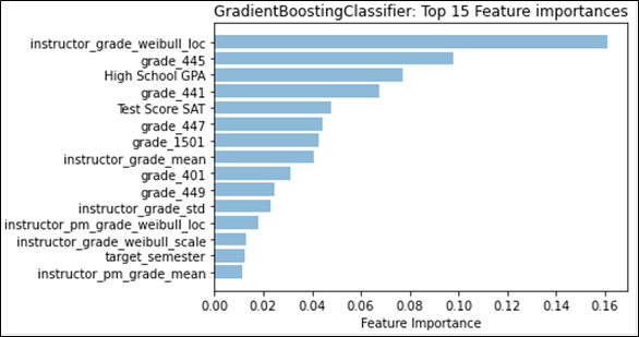
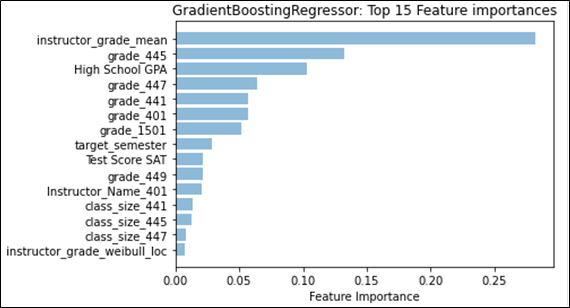
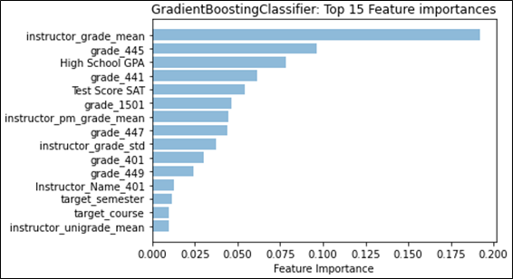
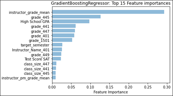
Referring to Figure 1, we see that for classification, “instructor_grade_weibull_loc” has the largest feature weight; this feature describes one of the parameters for the fitted Weibull distribution, namely “location.” Location for the Weibull distribution is analogous to the mean for the normal distribution. In our case, the “instructor_grade_weibull_loc” summarizes the instructor’s grades for the target course across all semesters in the dataset before the target semester. Similarly, for regression, the instructor’s mean grade for the target course instead factors as the most-predictive feature. With grading strategies like curving or partial credit, it is easy to see how the instructor’s (subjective) grading style can affect the final grade. We also notice that the difference in contribution between the top-two features is quite large. The difference between the top contributor in classification (approx. 0.16) and the second contributor (approx. 0.10) greatly exceeds the difference between the remaining consecutive features (0.02). A similar effect can be seen in regression, where the top contributor has a feature importance that is more than double the second feature. This shows that the grades that an instructor is likely to give in a target course is a strong predictor of what kind of grade the student is likely to achieve in the target course. We examine the distribution type in more detail in Section 5.3.
Six out of the top 10 features are grades that the student achieved in the given course number. In this case, all 6 courses are mandatory (out of 8 total) for CS majors to take at the university. The second-most predictive feature for both classification and regression are also for the same mandatory course. It seems intuitive that these courses would provide insight into how students would do in future courses, emphasized by the idea that the curriculum requires students to take these mandatory courses first. However, it is likely that the importance of each course is inflated simply because of the mandatory requirement, and as a result provides the initial information that is necessary to predict courses earlier in a student’s undergraduate career. This type of result may not hold as strongly in a major that does not provide a mandatory course schedule.
High school GPA rounds out the top-three. This is consistent with previous literature that indicates that the overall grades received by an incoming student can predict success at the university level [16], from student retention (e.g. [12]) to higher freshmen grades (e.g. [10]). The combined verbal and math score for the SAT also stands out as one of the top features, but is not as predictive as high school GPA, which consistent with the literature [3]. Typically, college-preparedness features are assumed to only have the most impact upon arrival at the university, which is why the typical benchmark for student success that uses these features tends to be freshmen grades. From our work here, it may suggest that these features are more representative of student success throughout the student’s undergraduate career.
While not as predictive as some of the top features, “target_semester” appears as a top-15 feature for both classification and regression, which may suggest that the timing in which a student takes a particular course in their major in relation with other major courses is correlated to their success. However, it is not clear what the causal link may be; it is reasonable to hypothesize that students who take courses in close succession are likely to do better, but it may also be the case that students who do better are more likely to take courses in quick succession. There is also a likelihood that delays in taking courses due to repeating failed courses may be captured by this feature.
5.2 Feature Type Comparisons
To provide a proper comparison between feature types (each of which is detailed in Section 4.1), we choose to retrain and retest GradientBoost over each feature type by itself to contrast them with the model trained over all feature types. Given our goal in this paper is to determine the impact that instructor features have on grade prediction models, we also compare a model trained with all feature types except for Instructor Characteristics. We perform the same validation techniques as mentioned in Section 4.3 (5-fold soft vote for classification and 5-run average for regression).
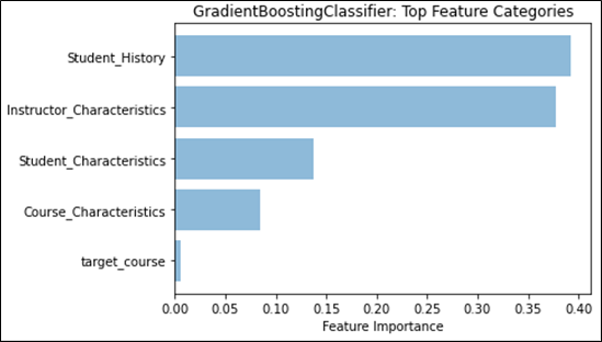
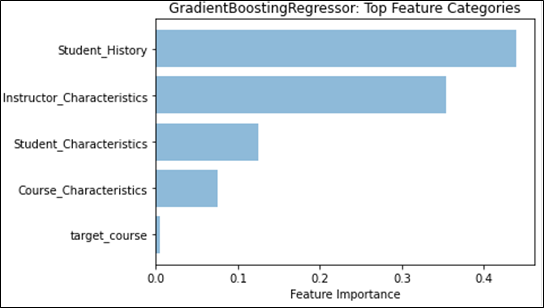
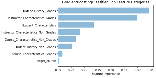
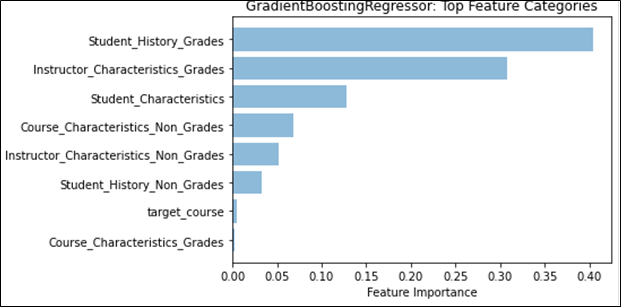
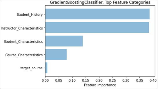
We can see that the Student Grade History feature category continues to be the main feature type for student grade prediction. From Table 5, we note that for all comparison metrics, either the classifier or regressor trained with only Student Grade History features outperforms all other singular feature type trained models. Furthermore, when training GradientBoost over all features, Figure 2 shows that Student Grade History features provides the highest feature weight among all categories. Along with the discussion about course grades from the section above, this provides further evidence to confirm previous research indicating that past student grades are a good predictor for future grades.
Instructor Characteristics comes closely in second, on many of the same angles presented for Student Grade History. From Table 5, we note that the classifier and regressor trained with only Instructor Characteristics has a similar performance with Student Characteristics and outperforms Course Characteristics on all comparison metrics. In terms of feature weights, we also see in Figure 2 that Instructor Characteristics comes closely in second and is almost on par with Student Grade History in the classification task. While individually, an instructor’s grade distribution retains the highest feature weight (as seen in Figure 1), collectively, they still fall short of Student Grade History.
| Feature Category |
Model | Training | Testing
| ||||
|---|---|---|---|---|---|---|---|
| Weighted F1 | MAE | RMSE | Weighted F1 | MAE | RMSE | ||
| Student Characteristics | GradClass | 0.41 | 0.75 | 1.18 | 0.40 | 0.77 | 1.18 |
| GradReg | 0.30 | 0.77 | 1.01 | 0.29 | 0.77 | 1.01 | |
| Grade History | GradClass | 0.46 | 0.70 | 1.13 | 0.44 | 0.74 | 1.16 |
| GradReg | 0.37 | 0.70 | 0.93 | 0.36 | 0.72 | 0.94 | |
| Course Characteristics | GradClass | 0.39 | 0.79 | 1.22 | 0.36 | 0.83 | 1.24 |
| GradReg | 0.23 | 0.80 | 1.03 | 0.22 | 0.81 | 1.04 | |
| Instructor Characteristics | GradClass | 0.42 | 0.75 | 1.17 | 0.38 | 0.79 | 1.19 |
| GradReg | 0.29 | 0.78 | 1.01 | 0.29 | 0.79 | 1.03 | |
| Student + Grade + Course Characteristics | GradClass | 0.49 | 0.65 | 1.06 | 0.46 | 0.68 | 1.09 |
| GradReg | 0.41 | 0.68 | 0.91 | 0.40 | 0.70 | 0.94 | |
| All Features | GradClass | 0.53 | 0.60 | 1.02 | 0.50 | 0.63 | 1.03 |
| GradReg | 0.44 | 0.66 | 0.88 | 0.44 | 0.66 | 0.89 | |
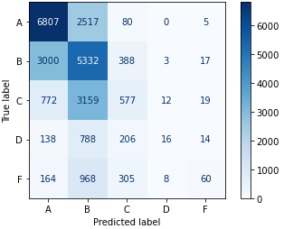
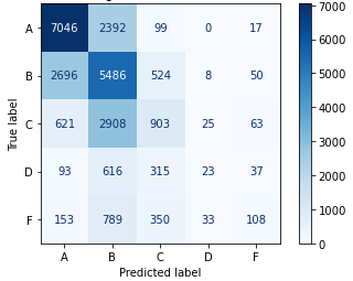
To provide assurance that Instructor Characteristics helps with student grade prediction, we compared two feature sets when training and testing GradientBoost, one trained with all features, and one trained without Instructor Characteristics. Results in Table 5 indicate that for both classification and regression, GradientBoost performs better when Instructor Characteristic features are included. We further examine the classification confusion matrix in Figure 3; in comparing Figures 3a and 3b, we see that adding Instructor Characteristics does have a general positive effect on the accuracy of the classification, given that the number of correct classifications (numbers on the diagonal) increases, and the number of incorrect classifications (numbers not on the diagonal) decreases. Furthermore, we also note that the total misclassifications that are one grade away (adjacent to the diagonal) increases, while the total misclassifications elsewhere decreases. This further confirms that instructor features do have a positive impact in overall classification, not just in singularly increasing recall or precision.
5.3 Grade Distributions and Representation
We tested 103 different distribution types (implemented by SciPy [33]), as well as the logit-normal distribution [2], over the full dataset to determine which kind of distribution best represents the grades’ GPA-equivalent values. We evaluated each distribution using the sum of squared error, and the best fit was the Weibull distribution, which can be represented by three parameters, location, shape, and scale. For every relevant grade distribution, we fit a Weibull distribution to the corresponding grouping, and each parameter was then considered an independent feature. Overall, 10 features were derived from the normal distribution, and 15 were derived from the Weibull distribution. In addition, out of the 25 total features, 5 were Course Characteristics (all grades ascribed to the course up to the target semester, regardless of instructor), and 20 were Instructor Characteristics.
| Feature Set | Distribution Type |
Model | Training | Testing
| ||||
|---|---|---|---|---|---|---|---|---|
| Weighted F1 | MAE | RMSE | Weighted F1 | MAE | RMSE | |||
All Features |
None | GradClass | 0.50 | 0.64 | 1.06 | 0.46 | 0.68 | 1.09 |
| GradReg | 0.40 | 0.69 | 0.91 | 0.39 | 0.70 | 0.93 | ||
| Weibull Only | GradClass | 0.53 | 0.61 | 1.02 | 0.49 | 0.64 | 1.05 | |
| GradReg | 0.44 | 0.66 | 0.88 | 0.43 | 0.67 | 0.90 | ||
| Normal Only | GradClass | 0.53 | 0.60 | 1.01 | 0.49 | 0.64 | 1.05 | |
| GradReg | 0.44 | 0.66 | 0.88 | 0.44 | 0.66 | 0.89 | ||
|
Both | GradClass | 0.53 | 0.60 | 1.02 | 0.50 | 0.63 | 1.04 | |
| GradReg | 0.44 | 0.66 | 0.88 | 0.44 | 0.66 | 0.89 | ||
| Instructor Characteristics Only |
None | GradClass | 0.41 | 0.79 | 1.23 | 0.37 | 0.82 | 1.24 |
| GradReg | 0.20 | 0.80 | 1.03 | 0.20 | 0.81 | 1.04 | ||
| Weibull Only | GradClass | 0.42 | 0.75 | 1.16 | 0.39 | 0.78 | 1.18 | |
| GradReg | 0.29 | 0.78 | 1.02 | 0.29 | 0.78 | 1.02 | ||
| Normal Only | GradClass | 0.41 | 0.75 | 1.17 | 0.39 | 0.78 | 1.19 | |
| GradReg | 0.29 | 0.78 | 1.01 | 0.29 | 0.78 | 1.02 | ||
|
Both | GradClass | 0.42 | 0.74 | 1.16 | 0.39 | 0.78 | 1.19 | |
| GradReg | 0.30 | 0.78 | 1.01 | 0.29 | 0.79 | 1.03 | ||
There is some controversy about using the normal distribution for representing grades [11], so we briefly investigated the effect of having only the Weibull distribution or the normal distribution represent the grades. We retrained and retested the GradientBoost classifier and regressor with the same procedure in Section 4.3 (5-fold soft vote for classification and 5-run average for regression), both of which are reported in Table 6. From the results, having at least one representation of grade distribution provides some benefit over not having a representation at all, with no difference in performance between the distribution type. Having both provides little-to-no benefit, so it is easy to conclude that it does not matter which grade distribution representation is included, so long as a representation is expressed in the feature set.
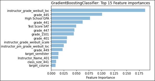
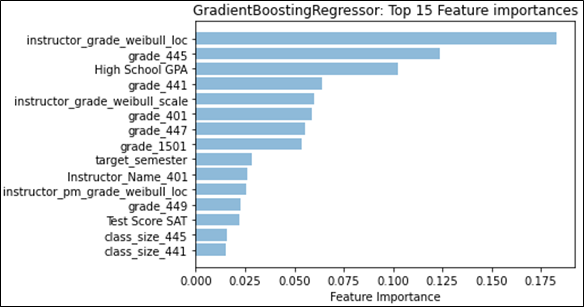
Feature weights provided a different angle with which to determine any effects that may stem from the different kinds of distributions. We first examined the effect that historical grades and their distributions had on future grade prediction by examining the weights of those features separately from the main categories. Figure 4 shows that Student Grade History grades and Instructor Category grade distributions would be the top two feature categories, if they were on their own. We then compared the effect that having a singular distribution type has on feature weights, to see if there were any notable changes. Figure 5 shows that no matter which distribution type is being used, the mean or the Weibull distribution’s analogous parameter, location, will remain the top feature overall. However, it is important to note that for the regression task, GradientBoost assigns a much higher weight to the mean than to Weibull’s location parameter, and even the sum of all three Weibull distribution parameter feature weights, indicating a stronger preference for the normal distribution for regression. We also see this effect appear when both distributions are used, as seen in Figure 1; classification prefers Weibull’s location parameter, while regression prefers the mean. This may provide evidence that the mean captures information that overlaps with more features, more so than the Weibull distribution, given that the performance does not noticeably increase. As for feature categories, no placement change was noted. However, in Figure 6, we see that the total feature weight for Instructor Characteristics is almost on par with Student Grade History during classification, further emphasizing the role that the normal distribution can have on predictive models.
5.4 Implications
While our model still has room for improvement for student grade prediction, there are several key items that can be derived from this research.
First, instructor-based features have a place in student grade prediction. The Student Grade History feature type continues to provide the most predictive power for grade prediction, and Instructor Characteristics follows closely behind in second place, while other feature types lag behind.
Second, the distribution of instructor grades is an important feature class to include in future student grade prediction models. It may not matter what kind of grade distribution representation is needed, despite prior research into the “appropriate” distribution, but the parameters for the normal distribution may assist with feature selection, given its high weight in the regression task.
Third, given the strong importance of the distribution of grades that an instructor assigns in their courses, more research is needed to determine the best way to either reduce the impact that instructors have on final grades through teaching ability or subjective measures, or conversely, ensuring that the grades that instructors assigned are truly unbiased and dependent only on the student’s performance in the course. Indeed, it is a long-standing question about the reliability and validity of grades themselves as a measurement of knowledge, given the significant variability in assigning them [7]. One could attempt to expose some of these subjective items by measuring student satisfaction for the instructor, characterizing the instructor’s teaching style, or determining the instructor’s efficacy when utilizing learning management systems, but those would all require additional data collection beyond what a university might readily have access to.
Lastly, there is still significant room for improvement in explainable student grade prediction. One area where significant work has been done is in Knowledge Tracing to diagnose student issues while they complete a course. Intuitively, understanding how students are doing within a course will ultimately determine how students will do overall, given the knowledge dependency within the course, which is especially important in STEM majors. While Knowledge Tracing does provides additional insight, the effort for training a model significantly increases due to the variation in course content material; it remains to be seen if Knowledge Tracing-adjacent or domain-agnostic Knowledge Tracing features can be generated to assist with generalized student grade prediction without introducing an extra heavy burden.
6. CONCLUSION
In attempting to characterize the relationship between instructor features and predicting a student’s grade, we first enumerated the feature space in grade prediction, with additional emphasis on generating features that describe an instructor’s history and experience in teaching. These features were then extracted from over 13 years and thousands of students’ grade records from a large, public, American university, and used to train and test several supervised ML models. From our experiments, the GradientBoost algorithm, both as classifier and regressor, has the best performance when compared with other supervised ML models.
We then used GradientBoost as our comparison algorithm between different features and feature types, in order to determine the utility of features that define an instructor in a grade prediction model. First, we noted that the distribution of grades that an instructor gives, specifically the mean or the Weibull distribution’s analogous parameter, location, is a major factor in grade prediction. Upon further review, it was found that the distribution representation does not make a major difference in the performance of the model. We then grouped features by type and found that Instructor Characteristics has the second-highest combined feature weight, closely behind Student Grade History. We further trained GradientBoost with and without Instructor Characteristics, and found that Instructor Characteristics contributed to better predictions of student grades for both classification and regression. Therefore, we strongly insist that future ML models should include features that describe Instructor Characteristics, or at the very least, features that describe the distribution of grades that an instructor assigns to a course.
References
- Yupei Zhang et al. “Undergraduate Grade Prediction in Chinese Higher Education Using Convolutional Neural Networks”. In: Proceedings of the 11th International Learning Analytics and Knowledge Conference (LAK 2021). Online Everywhere, 2021, pp. 462–468.
- Audrey Tedja Widjaja, Lei Wang, and Truong Trong Nghia. “Next-Term Grade Prediction: A Machine Learning Approach”. In: Proceedings of The 13th International Conference on Educational Data Mining (EDM 2020). Fully Virtual, 2020, pp. 700–703.
-
Pauli Virtanen et al. “SciPy 1.0: Fundamental
Algorithms for Scientific Computing in Python”.
In: Nature Methods 17 (2020), pp. 261–272. doi:
10.1038/s41592-019-0686-2. - Mack Sweeney et al. “Next-Term Student Performance Prediction: A Recommender Systems Approach”. In: Journal of Educational Data Mining 8.1 (2016), pp. 22–51.
- Sergi Rovira, Eloi Puertas, and Laura Igual. “Data-driven system to predict academic grades and dropout”. In: PLoS ONE 12.2 (2017), pp. 1–21.
- Steffen Rendle. “Factorization Machines with libFM”. In: ACM Transactions on Intelligent Systems and Technology 2.3 (2012), pp. 1–22.
- Steffen Rendle. “Factorization Machines”. In: Proceedings of the 2010 IEEE International Conference on Data Mining (ICDM 2010). Sydney, Australia, 2010, pp. 995–1000.
- Zhiyun Ren et al. “Grade Prediction with Neural Collaborative Filtering”. In: Proceedings of the 2019 IEEE International Conference on Data Science and Advanced Analytics (DSAA). Washington, DC, 2019, pp. 1–10.
- Zhiyun Ren et al. “Grade Prediction Based on Cumulative Knowledge and Co-taken Courses”. In: Proceedings of The 12th International Conference on Educational Data Mining (EDM 2019). Montréal, Canada, 2019, pp. 158–167.
- Zhiyun Ren, Huzefa Rangwala, and Aditya Johri. “Predicting Performance on MOOC Assessments using Multi-Regression Models”. In: Proceedings of the Ninth International Conference on Educational Data Mining (EDM 2016). Raleigh, North Carolina, 2016, pp. 484–489.
- Agoritsa Polyzou and George Karypis. “Grade Prediction with Course and Student Specific Models”. In: Proceedings of the 20th Pacific Asia Conference on Knowledge Discovery and Data Mining (PAKDD) 2016. Auckland, New Zealand, 2016, pp. 89–101.
- Agoritsa Polyzou. “Models and Algorithms for Performance Prediction and Course Recommendation in Higher Education”. Ph.D. diss. Minneapolis, Minnesota: University of Minnesota, 2020.
- F. Pedregosa et al. “Scikit-learn: Machine Learning in Python”. In: Journal of Machine Learning Research 12 (2011), pp. 2825–2830.
- Phil Pavlik Jr. et al. “Using Item-type Performance Covariance to Improve the Skill Model of an Existing Tutor”. In: Proceedings of the First International Conference on Educational Data Mining (EDM 2008). Montréal, Canada, 2008, pp. 77–86.
- Behrooz Parhami. “Voting algorithms”. In: IEEE Transactions on Reliability 43.4 (1994), pp. 617–629.
-
Isaac M. Opper. Teachers
Matter: Understanding Teachers’ Impact on Student
Achievement. Santa Monica, CA: RAND Corporation,
2019. doi:
10.7249/RR4312. - Sara Morsy and George Karypis. “Cumulative Knowledge-based Regression Models for Next-term Grade Prediction”. In: Proceedings of the 2017 SIAM International Conference on Data Mining (SDM). Houston, Texas, 2017, pp. 552–560.
-
Corey Lynch. pyFM.
https://github.com/coreylynch/pyFM. 2018. - Andrew E. Krumm et al. “A Learning Management System-Based Early Warning System for Academic Advising in Undergraduate Engineering”. In: Learning Analytics: From Research to Practice. Ed. by Johann Ari Larusson and Brandon White. 1st ed. Springer-Verlag, 2014. Chap. 6, pp. 103–119.
- Eunhee Kim et al. “Personal factors impacting college student success: Constructing college learning effectiveness inventory (CLEI)”. In: College Student Journal 44.1 (2010), pp. 112–126.
-
Common Core Standards Initiative. Mathematics
standards.
http://www.corestandards.org/Math/. Accessed: 2021-09-08. 2021. - Qian Hu et al. “Enriching Course-Specific Regression Models with Content Features for Grade Prediction”. In: Proceedings of the 4th IEEE International Conference on Data Science and Advanced Analytics (DSSA2017). Tokyo, Japan, 2017, pp. 462–468.
- Caitlin Holman et al. “Planning for Success: How Students Use a Grade Prediction Tool to Win Their Classes”. In: Proceedings of the Fifth International Conference on Learning Analytics And Knowledge (LAK 2015). Poughkeepsie, New York, 2015, pp. 260–264.
- Brady P Gaskins. “A ten-year study of the conditional effects on student success in the first year of college”. PhD thesis. Bowling Green State University, 2009.
- Lynn Fendler and Irfan Muzaffar. “The history of the bell curve: Sorting and the idea of normal”. In: Educational Theory 58.1 (2008), pp. 63–82.
- Elchanan Cohn et al. “Determinants of undergraduate GPAs: SAT scores, high-school GPA and high-school rank”. In: Economics of education review 23.6 (2004), pp. 577–586.
-
CNN. Pushcart classes help break gang chain.
http://www.cnn.com/2009/LIVING/wayoflife/03/05/heroes.efren.penaflorida/index.html. Accessed: 2021-09-08. 2009. - Nitesh V Chawla et al. “SMOTE: synthetic minority over-sampling technique”. In: Journal of artificial intelligence research 16 (2002), pp. 321–357.
- Susan M Brookhart et al. “A Century of Grading Research: Meaning and Value in the Most Common Educational Measure”. In: Review of Educational Research 86.4 (2016), pp. 803–848.
- Hall P Beck and William D Davidson. “Establishing an early warning system: Predicting low grades in college students from survey of academic orientations scores”. In: Research in Higher Education 42.6 (2001), pp. 709–723.
- Michael Backenköhler et al. “Data-Driven Approach Towards a Personalized Curriculum”. In: Proceedings of the Eleventh International Conference on Educational Data Mining (EDM 2018). Buffalo, New York, 2018, pp. 246–251.
- Ken Ayo Azubuike and Orji Friday Oko. “IMPACT OF TEACHERS’ MOTIVATION ON THE ACADEMIC PERFORMANCE OF STUDENTS: IMPLICATIONS FOR SCHOOL ADMINISTRATION”. In: National Journal of Educational Leadership 3 (2016), pp. 91–99.
- A.W. Astin. What Matters in College?: Four Critical Years Revisited. Jossey-Bass higher and adult education series. Wiley, 1997. isbn: 9781555424923.
- Noah Arthurs et al. “Grades Are Not Normal: Improving Exam Score Models Using the Logit-Normal Distribution.” In: Proceedings of The 12th International Conference on Educational Data Mining (EDM 2019). Montréal, Canada, 2019, pp. 252–257.
- Rahaf Alamri and Basma Alharbi. “Explainable Student Performance Prediction Models: A Systematic Review”. In: IEEE Access 9 (2021), pp. 33132–33143.
1The categories and corresponding GPA values can be found in Table 3.
2We define half grades to be when the grade changes by one step (e.g., from A to A or B+ to A-), while a full grade change is when the letter changes (e.g., from A to B)
3The SAT and ACT are common standardized exams that high school students take for entry to an American undergraduate program. For this university, these scores are not required, and are given 0 if no score is provided. Note that 0 is not a valid score for either exam.
© 2022 Copyright is held by the author(s). This work is distributed under the Creative Commons Attribution-NonCommercial-NoDerivatives 4.0 International (CC BY-NC-ND 4.0) license.