ABSTRACT
In this paper, we propose a novel approach to combine domain modelling and student modelling techniques in a single, automated pipeline which does not require expert knowledge and can be used to predict future student performance. Domain modelling techniques map questions to concepts and student modelling techniques generate a mastery score for a concept. We conducted an evaluation using six large datasets from a Python programming course, evaluating the performance of different domain and student modelling techniques. The results showed that it is possible to develop a successful and fully automated pipeline which learns from raw data. The best results were achieved using alternating least squares on hill-climbing Q-matrices as domain modelling and exponential moving average as student modelling. This method outperformed all baselines in terms of accuracy and showed excellent run time.
Keywords
1. INTRODUCTION
The idea of mastery learning was first proposed by Bloom [3] as an educational philosophy based on the belief that nearly all students can master a studied subject when given enough time and support. Nowadays, the term more commonly refers to an educational approach where test questions assess certain concepts and a mastery of prerequisite concepts is required before moving to harder concepts [11]. A concept or skill (we use this terms interchangeably) can be thought of as a unit of knowledge that is assessed by a question; for example, a mathematics question might assess the concepts of "addition" and "subtraction", or a programming question might assess the concepts of "print statements" and "strings" [7]. A common application of this approach is for task sequencing in intelligent tutoring systems, where remedial questions for students are selected based on concepts they are weak at [11]. These approaches can also be used for providing automated feedback to students and hint generation [8]. But how do we know the full set of concepts in a set of questions? How do we know which questions assess which concepts? How do we measure the extent to which a student has "mastered" each concept? There are two distinct but related fields of research that attempt to answer these questions—domain modelling and student modelling [12].
Domain modelling is concerned with knowing the full set of concepts in a set of questions, and knowing which questions assess which concepts. This mapping of questions to concepts can be represented as a Q-matrix, a matrix, where each entry is either 1 or 0, with 1 representing that the question in the row assesses the concept in the column [13]. Several previous studies have proposed methods for generating a Q-matrix based on student performance data on question sets; e.g. Barnes [2] introduced a hill-climbing algorithm, and Desmarais et al. [5] proposed a method in which Alternating Least Squares (ALS) method is used to refine an expert-designed Q-matrix.
Student modelling is concerned with measuring the extent to which a student has mastered a concept, or how to generate a mastery score. For instance, Corbett et al. [4] introduced Bayesian Knowledge Tracing, which uses a Markov model with two hidden states (a concept is either ’known’ or ’unknown’ by a student), with further refinements to this technique proposed by Pardos et al. [9] and Yudelson et al. [14].
In this paper, we aim to combine domain and student modelling in a single, automated pipeline. In other words, is it possible to go from domain modelling to student modelling in a single pipeline on a single dataset, and thus predict future student performance? Solving this problem would be of significant benefit for intelligent tutoring systems, for example for task sequencing. Using only historic student performance data on questions, it would be possible to automatically generate a mapping between questions and concepts, and generate a mastery score for each student for each concept. This can then be used to sequence remedial tasks for students, i.e., for recommending tasks which assess the concepts at which the students were the weakest, with minimal human input.
This study attempts to explore this question, and has three main contributions. First, it provides an implementation and analysis of a pipeline that includes different combinations of three domain modelling and three student modelling techniques, where the results are based on predicting future student performance using the mastery score. Second, it performs this analysis on large datasets from an online programming course - 6 datasets across 2 years with 3 levels of expertise (beginners, intermediate and advanced), with a total of 144 questions and 28,466 students - demonstrating consistent results across all datasets. Third, it introduces a new Q-matrix generation technique - ALS on Hill-Climbing Q-matrix. The results show that the proposed technique is the most successful student modeling - it is best combinations of domain and student modelling in 5/6 cases.
2. RELATED WORK
2.1 Domain Modelling (Q-matrix Generation Algorithms)
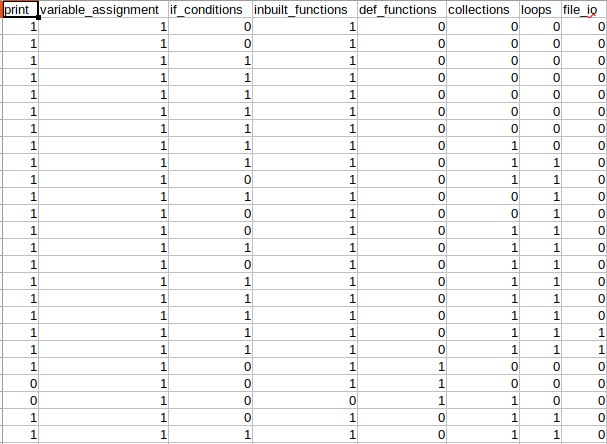
A Q-matrix is a mapping between questions in a set, and the skills or concepts that they assess [13]. An example is shown in Fig. 1. Such matrices are used to determine the probabilities that certain skills are learned by a student, and to select and sequence tasks in mastery learning environments. While Q-matrices are traditionally designed by experts, we have to consider disagreement between experts, the amount of time and effort needed to do this process manually, as well as disagreement between expert opinion and what students actually experience.
Barnes [2] introduced an algorithm that can derive a Q-matrix from student response data. The algorithm initializes a matrix ( being the number of students, the number of skills) with random values for each cell in range . Given the current Q-matrix, it computes, for each student, the binary knowledge states which best describe the student’s actual test responses. Then, hill-climbing is performed to improve the matrix given the current knowledge state estimate. This is repeated until convergence, and repeated for different numbers of concepts.
By contrast, Desmarais et al. [5] propose to let an expert design the initial Q-matrix, and then optimising via the ALS method. This is motivated by expressing the matrix of student responses ( being the number of students) as a product of two matrices and ; the Q matrix being an matrix as before, and the S matrix being a matrix that represents student mastery profiles. The ALS method minimizes the squared error with respect to and in an alternating fashion until convergence.
In this paper, we propose a new method which combines hill-climbing and ALS, called ALS on Hill-climbing Q-Matrix. It uses a hill-climbing algorithm to derive an initial Q-matrix, and then ALS to refine it. We evaluate the performance of three methods: Hill-climbing Q-matrix, ALS on Expert Q-matrix and ALS on Hill-climbing Q-matrix.
2.2 Student Modelling (Mastery Score Algorithms)
Once a Q-matrix is known, the students’ learning process can be described by modelling which skill is mastered at what time by which student.
Kelly et al. [6] conducted a study to determine the accuracy of two methods, namely -Consecutive Correct Responses (-CCR) and Knowledge Tracing (KT) [4] in detecting concept mastery in students. The study defined mastery of a concept as a binary attribute. -CCR is a simple algorithm that considers a skill mastered once a student gives consecutive correct responses on questions related to the skill. By contrast, KT models student knowledge as a latent variable in a Hidden Markov Model, with the parameters updated based on whether or not the student gets each question in a sequence of questions correct or wrong (more detail on this below). The algorithm computes the probability that a student has mastered a skill after each observation of a correct or incorrect answer. The study concluded by stating that 3-CCR was the better approach for next-problem correctness, and 5-CCR was the better approach for predicting performance on a transfer task, with both methods being more accurate than knowledge tracing.
However, -CCR has drawbacks which are not discussed in the paper. Consider two students who answered a sequence of 6 questions, and assume we consider 5-CCR, with the vectors representing the correctness of the answers of each student being and . 5-CCR would determine that both students have the same level of mastery, which can be argued is not true. One way to mitigate this is to introduce a method where more recent answers carry more weight in determining the measure of mastery. The exponential moving average (EMA) technique [10] estimates the mastery of a student after answering the th question via the expression , where is if the student answered question correctly and , otherwise, and where is a weight for past states, with being a hyperparameter that controls how fast this weight decays into the past.
Corbett et al. [4] introduced the concept of Bayesian Knowledge Tracing (BKT). BKT assumes that a concept is a latent binary variable (either mastered or not mastered by a student) in a Hidden Markov Model, with observations also being binary (a student can get a question correct or incorrect). There are 4 parameters in this model; the probability that a student has mastered the skill prior to attempting the first question, the probability that a student will master the concept after one opportunity to apply the concept in a question, the probability that a student will get a question correct given they have not mastered a concept (’guess’), and the probability that a student will get a question incorrect given that they have mastered a concept (’slip’). One model is built for each concept , assuming that the concepts assessed in a given question are known.
In this paper, we will evaluate all three approaches: -CCR, EMA and BKT.
3. DATA AND PREPROCESSING
The data used in this study was provided by Grok Academy (groklearning.com) and comes from three online Python programming courses for high school students. In total it comes from 28,466 students and includes 144 questions. In this learning platform, students complete coding tasks and receive automated feedback in the form of passed test cases and feedback about the failed cases, e.g. comparison between the expected output and the student’s output.
Our study uses a total of 6 datasets from 2 years (2018 and 2019), with each year having one set of questions from 3 difficulty levels (beginners, intermediate and advanced). Table 1 summarises the dataset statistics.
| Questions | Students | |
|---|---|---|
| Beginners-2018 | 29 | 7956 |
| Intermediate-2018 | 25 | 4756 |
| Advanced-2018 | 22 | 731 |
| Beginners-2019 | 28 | 8662 |
| Intermediate-2019 | 25 | 5423 |
| Advanced-2019 | 15 | 938 |
For each student, we collected a ’trace’ of all their submissions on each question. A student may submit solutions multiple times for a question, each time getting feedback in terms of expected vs actual program output, and the number of test cases passed. However, domain and student modelling approaches typically require a single binary value of correctness for each student on each question. To obtain such a value, we used 1 if the average number of passed test cases per submission exceeded the median, and 0, otherwise. For example, if a student attempts a question 3 times and passes 0/10, 5/10 then 10/10 test cases, then we take the average over the 3 attempts, which is 5/10, and map this to 1 if 5/10 is larger than the median value over all students for this question.
4. METHOD
There are two main steps, namely domain modelling and student modelling. The first step infers the relation between questions and concepts in a form of Q-matrix. The second step builds a model to predict a student’s future performance based on their past responses.
We consider three algorithms for domain modelling, namely Hill-climbing Q-matrix [2], ALS on Expert Q-matrix [5], and ALS initialized with Hill-climbing Q-matrix. The last one is our proposed method and it combines hill-climbing and ALS algorithms. Further, we consider three algorithms for student modelling, namely -CRR, EMA, and BKT. The pipeline for each combination of domain modelling and student modelling components is as follows.
First, infer a Q-matrix using the domain modelling component. Second, for each student, extract one sequence of correct and wrong responses to questions that are related to that skill. Finally, use the student modelling component to model the mastery of each student for each skill.
For prediction, we consider the mastery score after responding to the th question and predict a successful response if the mastery score exceeds a threshold. Our evaluation measure is the RMSE between the mastery scores and the actual responses.
5. EXPERIMENTAL SETUP
Combining each domain modelling algorithm (Hill-climbing Q-matrix, ALS on Expert Q-matrix, ALS on Hill-climbing Q-matrix) with each student modelling algorithm (-CCR, EMA, BKT) yields nine combinations. We evaluate each combination on each data set from Table 1. For brevity and lack of space reasons, we discuss in detail the 2018 datasets but provide only the best results for the 2019 datasets.
Using hill-climbing, we generate 10 matrices for each dataset with to concepts. The runtime needed for the matrix generation is shown in Table 2.
| Dataset | Hill-climbing Q-matrix Runtime |
|---|---|
| Beginners-2018 | 5 hours |
| Intermediate-2018 | 4 hours |
| Advanced-2018 | 30 minutes |
| Beginners-2019 | 7 hours |
| Intermediate-2019 | 5 hours |
| Advanced-2019 | 45 minutes |
To evaluate the student modelling, we use five-fold cross validation over students. For -CCR and EMA, we also evaluate the results for different hyperparameter values: from to and from to .
Additionally, we compare the performance with three baselines, namely random guessing (random), predicting the majority label for each question (majority), and BKT with a single concept per question (BKT-1).
All six techniques were implemented in Python. For hill-climbing, ALS, -CCR, and EMA we used our own implementation, and for BKT we used the pybkt toolbox [1].
6. EXPERIMENTAL RESULTS
6.1 Beginners-2018
The performance of the three baselines on the 2018 datasets is shown in Table 3. We can see that the most accurate baseline on all 3 datsets is BKT-1, followed by majority and random.
| Baseline Method | beginner | intermediate | advanced |
|---|---|---|---|
| random | 0.7065 | 0.7054 | 0.7131 |
| majority | 0.6576 | 0.6447 | 0.5270 |
| BKT-1 | 0.4899 | 0.4880 | 0.4280 |
Table 4 shows the RMSE for BKT, EMA, and -CCR on the Beginners-2018 dataset for Q-matrices that were generated via hill-climbing; the best results are shown in bold. For EMA and -CCR, we only report the results for the best-performing values of and (the results for other hyperparameter values are shown in Table 5). Each row represents the results obtained for a certain number of concepts. Here, it is interesting to see that, for EMA and -CCR, the best Q-matrix is the one with only 1 concept, while, for BKT, the best Q-matrix had 9 concepts. The RMSE stays relatively stable for the different Q-matrices for BKT. For BKT and -CCR, the RMSE stays relatively stable only for Q-matrices with 3 concepts and above. The last row of the table shows the prediction runtime; we can see that all methods were fast and had similar prediction runtime - 48-54 seconds.
| n_con | BKT | EMA (, RMSE) | -CCR (, RMSE) |
|---|---|---|---|
| 1 | 0.4453 | 0.1, 0.1487 | 1, 0.1482 |
| 2 | 0.4316 | 0.1, 0.1588 | 1, 0.1594 |
| 3 | 0.4352 | 0.1, 0.2476 | 1, 0.2484 |
| 4 | 0.4391 | 0.1, 0.2261 | 1, 0.2276 |
| 5 | 0.4368 | 0.1, 0.2274 | 1, 0.2286 |
| 6 | 0.4351 | 0.1, 0.2280 | 1, 0.2293 |
| 7 | 0.4340 | 0.1, 0.2193 | 1, 0.2208 |
| 8 | 0.4318 | 0.1, 0.2114 | 1, 0.2131 |
| 9 | 0.4305 | 0.1, 0.2463 | 1, 0.2491 |
| 10 | 0.4309 | 0.1, 0.2389 | 1, 0.2417 |
| (sec) | 54.1 | 49.7 | 48.5 |
It is also interesting to note that, regardless of the number of concepts, and are the best-performing hyperparamters for EMA and -CCR, respectively (see Table 4). In other words, it was always best to predict the performance on the next question based on the question immediately before it. Table 5 provides more details about the impact of the hyperparameters and on the RMSE. We see a clear trend: as and increase, RMSE rises as well.
| (EMA) | RMSE | N (-CCR) | RMSE | |
|---|---|---|---|---|
| 0.1 | 0.1487 | 1 | 0.1482 | |
| 0.2 | 0.1624 | 2 | 0.1742 | |
| 0.3 | 0.1857 | 3 | 0.2068 | |
| 0.4 | 0.2148 | 4 | 0.2524 | |
| 0.5 | 0.2470 | 5 | 0.3067 | |
| 0.6 | 0.2809 | 6 | 0.3231 | |
| 0.7 | 0.3159 | 7 | 0.3059 | |
| 0.8 | 0.3523 | 8 | 0.3893 | |
| 0.9 | 0.3927 | 9 | 0.4257 |
Next, we evaluate BKT, EMA, and -CCR on the Q-matrix derived by ALS when initialized with an expert Q-matrix. The expert Q-matrix covers eight skills (refer to Fig. 1). Table 6 shows the results, indicating that EMA with performs best. Table 7 shows the performance of EMA and -CCR for different hyperparameter choices. For -CCR we observe the same trend as before, for EMA we observe that low -values generally perform better, with a minimum at .
| n_con | BKT | EMA (, RMSE) | -CCR (, RMSE) |
|---|---|---|---|
| 8 | 0.3908 | 0.3, 0.1874 | 1, 0.2176 |
| (sec) | 12.3 | 6.78 | 6.24 |
| (EMA) | RMSE | N (-CCR) | RMSE | |
|---|---|---|---|---|
| 0.3 | 0.1874 | 1 | 0.2176 | |
| 0.4 | 0.1874 | 2 | 0.2468 | |
| 0.2 | 0.1905 | 3 | 0.2725 | |
| 0.5 | 0.1909 | 4 | 0.2908 | |
| 0.1 | 0.1966 | 5 | 0.3086 | |
| 0.6 | 0.1986 | 6 | 0.3254 | |
| 0.7 | 0.2122 | 7 | 0.3373 | |
| 0.8 | 0.2340 | 8 | 0.3497 | |
| 0.9 | 0.2676 | 9 | 0.3553 |
Finally, we evaluate BKT, EMA, and -CCR on the Q-matrix derived by ALS when initialized with a hill-climbing Q-matrix. Table 8 shows the results. Again, EMA with performs best. Indeed, the results for EMA with are better than any other result we obtained across all domain modelling approaches. Interestingly, different values are optimal, depending on the number of concepts.
| n_con | BKT | EMA (, RMSE) | -CCR (, RMSE) |
|---|---|---|---|
| 1 | 0.4262 | 0.3, 0.1319 | 1, 0.1482 |
| 2 | 0.4054 | 0.5, 0.2164 | 1, 0.2507 |
| 3 | 0.4196 | 0.4, 0.1937 | 1, 0.2220 |
| 4 | 0.4260 | 0.3, 0.1760 | 1, 0.1901 |
| 5 | 0.4210 | 0.3, 0.1963 | 1, 0.2103 |
| 6 | 0.4232 | 0.2, 0.2094 | 1, 0.2196 |
| 7 | 0.4199 | 0.3, 0.2216 | 1, 0.2331 |
| 8 | 0.4231 | 0.3, 0.1714 | 1, 0.1861 |
| 9 | 0.4215 | 0.4, 0.1829 | 1, 0.2017 |
| 10 | 0.4214 | 0.4, 0.1945 | 1, 0.2129 |
| (sec) | 53.2 | 55.8 | 52.1 |
| (EMA) | RMSE | N (-CCR) | RMSE | |
|---|---|---|---|---|
| 0.3 | 0.1319 | 1 | 0.1482 | |
| 0.4 | 0.1327 | 2 | 0.1542 | |
| 0.2 | 0.1350 | 3 | 0.1580 | |
| 0.5 | 0.1396 | 4 | 0.1627 | |
| 0.1 | 0.1407 | 5 | 0.1641 | |
| 0.6 | 0.1556 | 6 | 0.1898 | |
| 0.7 | 0.1839 | 7 | 0.1953 | |
| 0.8 | 0.2289 | 8 | 0.2106 | |
| 0.9 | 0.2971 | 9 | 0.2348 |
In Table 9, we see that the RMSE of -CCR steadily worsens as increases. By contrast, the RMSE for EMA has a minimum at and increases for smaller or larger values.
6.2 Intermediate-2018
| n_con | BKT | EMA (, RMSE) | -CCR (, RMSE) |
|---|---|---|---|
| 1 | 0.4364 | 0.3, 0.3793 | 1, 0.3925 |
| 2 | 0.4037 | 0.3, 0.2977 | 1, 0.3083 |
| 3 | 0.4012 | 0.3, 0.2751 | 1, 0.2842 |
| 4 | 0.4050 | 0.3, 0.2610 | 1, 0.2726 |
| 5 | 0.4021 | 0.3, 0.2469 | 1, 0.2578 |
| 6 | 0.4045 | 0.3, 0.2433 | 1, 0.2541 |
| 7 | 0.4072 | 0.3, 0.2370 | 1, 0.2455 |
| 8 | 0.4068 | 0.3, 0.2306 | 1, 0.2389 |
| 9 | 0.4076 | 0.2, 0.2213 | 1, 0.2281 |
| 10 | 0.4060 | 0.2, 0.2175 | 1, 0.2242 |
| (sec) | 29.1 | 28.7 | 28 |
| (EMA) | RMSE | N (-CCR) | RMSE | |
|---|---|---|---|---|
| 0.2 | 0.2175 | 1 | 0.2242 | |
| 0.3 | 0.2176 | 2 | 0.2354 | |
| 0.1 | 0.2197 | 3 | 0.2429 | |
| 0.4 | 0.2203 | 4 | 0.2573 | |
| 0.5 | 0.2265 | 5 | 0.2758 | |
| 0.6 | 0.2373 | 6 | 0.2989 | |
| 0.7 | 0.2543 | 7 | 0.3217 | |
| 0.8 | 0.2793 | 8 | 0.3550 | |
| 0.9 | 0.3127 | 9 | 0.3870 |
| Skill | RMSE (BKT) | Skill | RMSE (EMA) | Skill | RMSE (-CCR) |
||
|---|---|---|---|---|---|---|---|
| 0 | 0.4366 | 0 | 0.3803 | 0 | 0.3925 | ||
| 1 | 0.3851 | 1 | 0.1844 | 1 | 0.1897 | ||
| 2 | 0.3970 | 2 | 0.2245 | 2 | 0.2282 | ||
| 3 | 0.2155 | 3 | 0.2339 | ||||
| 4 | 0.1790 | 4 | 0.1854 | ||||
| 5 | 0.2279 | 5 | 0.2339 | ||||
| 6 | 0.1856 | 6 | 0.1854 | ||||
| 7 | 0.1792 | 7 | 0.1854 | ||||
| 8 | 0.1137 | 8 | 0.1071 | ||||
| 9 | 0.1786 | 9 | 0.1854 |
From Table 10, it is interesting to note that the best models use Q-matrices with more concepts than seen in the previous dataset. For BKT, concepts is optimal, for EMA and -CCR it is 10 concepts. We also observe that, for EMA and -CCR, the more concepts we consider, the better performance gets (considering only the model with the best parameters), which is something that we did not observe in the previous dataset. While -CCR still selects 1 as the best N for all the Q-matrices, for EMA, most of the Q-matrices give either 0.3 or 0.2 as the best .
From Table 11, we can see that s of 0.1, 0.2 and 0.3 actually have very similar RMSE, with 0.4 and above steadily worsening in RMSE as increases. -CCR exhibits the pattern of RMSE worsening as N increases.
From Table 12, we see that, across all algorithms, the per-skill RMSE is not uniform at all. For example, for -CCR, skill 8 has an RMSE of 0.1071, while skill 0 has an RMSE of 0.3925. This can be interpreted as being caused by a large variance in student proficiency for certain skills, or that some skills are a lot harder to learn than others.
| n_con | BKT | EMA (, RMSE) | -CCR (, RMSE) |
|---|---|---|---|
| 8 | 0.3930 | 0.4, 0.2815 | 1, 0.1977 |
| (sec) | 8.01 | 4.95 | 4.33 |
| (EMA) | RMSE | N (-CCR) | RMSE | |
|---|---|---|---|---|
| 0.4 | 0.2815 | 1 | 0.1977 | |
| 0.5 | 0.2821 | 2 | 0.2009 | |
| 0.3 | 0.2821 | 3 | 0.2093 | |
| 0.2 | 0.2837 | 4 | 0.2145 | |
| 0.6 | 0.2844 | 5 | 0.2205 | |
| 0.1 | 0.2861 | 6 | 0.2247 | |
| 0.7 | 0.2899 | 7 | 0.2365 | |
| 0.8 | 0.3018 | 8 | 0.2481 | |
| 0.9 | 0.3265 | 9 | 0.2636 |
| Skill | RMSE (BKT) | Skill | RMSE (EMA) | Skill | RMSE (-CCR) |
||
|---|---|---|---|---|---|---|---|
| 0 | 0.4071 | 0 | 0.2691 | 0 | 0.1854 | ||
| 1 | 0.4105 | 1 | 0.1787 | 1 | 0.1854 | ||
| 2 | 0.4040 | 2 | 0.2079 | 2 | 0.2748 | ||
| 3 | 0.4061 | 3 | 0.1787 | 3 | 0.1854 | ||
| 4 | 0.3618 | 4 | 0.1788 | 4 | 0.1071 | ||
| 5 | 0.3776 | 5 | 0.1787 | 5 | 0.1854 | ||
| 6 | 0.3246 | 6 | 0.2079 | 6 | 0.1854 | ||
| 7 | 0.3374 | 7 | 0.5888 | 7 | 0.2280 |
From Table 13, we see that -CCR performs better than EMA. -CCR has chosen 1 as the best N, while EMA has 0.4 as the best .
From Table 14, we see that—while there is no pattern of worsening RMSE as increases for EMA—the first 7 values of have very very similar RMSE (differences lesser than 0.01). For -CCR we see that RMSE steadily worsens as increases. It is also interesting to note that the worst -CCR model (RMSE = 0.2636) performs better than the best EMA model (RMSE = 0.2815).
From Table 15, we see again that per-concept RMSE has high variance, more so with EMA and -CCR than BKT. Skill 7 has the highest RMSE when EMA is used, with an RMSE of 0.5888. Meanwhile, the skill with the worst RMSE for -CCR is skill 2 which only has an RMSE of 0.2748.
| n_con | BKT (RMSE) | EMA (, RMSE) | -CCR (, RMSE) |
|---|---|---|---|
| 1 | 0.4122 | 0.3, 0.1782 | 1, 0.1854 |
| 2 | 0.3955 | 0.4, 0.2341 | 1, 0.2549 |
| 3 | 0.4152 | 0.4, 0.2215 | 1, 0.2377 |
| 4 | 0.4117 | 0.6, 0.2608 | 1, 0.2952 |
| 5 | 0.4097 | 0.6, 0.2448 | 1, 0.2803 |
| 6 | 0.3990 | 0.5, 0.2453 | 1, 0.2693 |
| 7 | 0.3980 | 0.5, 0.2425 | 1, 0.2636 |
| 8 | 0.3995 | 0.5, 0.2593 | 1, 0.2865 |
| 9 | 0.3998 | 0.4, 0.2289 | 1, 0.2465 |
| 10 | 0.4050 | 0.4, 0.2397 | 1, 0.2621 |
| (sec) | 27.2 | 31.8 | 30 |
| (EMA) | RMSE | N (-CCR) | RMSE | |
|---|---|---|---|---|
| 0.3 | 0.1782 | 1 | 0.1854 | |
| 0.4 | 0.1787 | 2 | 0.1877 | |
| 0.2 | 0.1790 | 3 | 0.1889 | |
| 0.5 | 0.1801 | 4 | 0.1896 | |
| 0.1 | 0.1813 | 5 | 0.2198 | |
| 0.6 | 0.1830 | 6 | 0.2220 | |
| 0.7 | 0.1900 | 7 | 0.2248 | |
| 0.8 | 0.2092 | 8 | 0.2289 | |
| 0.9 | 0.2582 | 9 | 0.2335 |
It is interesting that, compared to the hill-climb Q-matrix without ALS refinement, the results in Table 16 show that ALS on Hill-climbing Q-matrix perform best when using Q-matrices with a smaller numbers of concepts.
From Table 17, we see the familiar pattern of -CCR selecting 1 to be the best N regardless of number of concepts, while EMA has many different values of being the best for different numbers of concepts. The largest found is 0.6 when we use the Q-matrix with 5 concepts - this yields an RMSE of 0.2608, which in fact is better than even the best BKT model by a decent margin.
6.3 Advanced-2018
| n_con | BKT | EMA (, RMSE) | -CCR (, RMSE) |
|---|---|---|---|
| 1 | 0.3573 | 0.1, 0.2117 | 2, 0.2115 |
| 2 | 0.3439 | 0.2, 0.2130 | 2, 0.2178 |
| 3 | 0.3580 | 0.2, 0.2215 | 1, 0.2254 |
| 4 | 0.3618 | 0.1, 0.2074 | 1, 0.2102 |
| 5 | 0.3557 | 0.1, 0.2086 | 1, 0.2114 |
| 6 | 0.3555 | 0.1, 0.2048 | 1, 0.2081 |
| 7 | 0.3581 | 0.2, 0.2308 | 1, 0.2346 |
| 8 | 0.3631 | 0.2, 0.2228 | 1, 0.2274 |
| 9 | 0.3636 | 0.2, 0.2191 | 1, 0.2233 |
| 10 | 0.3660 | 0.2, 0.2157 | 1, 0.2204 |
| (sec) | 6.22 | 5.55 | 5.33 |
| (EMA) | RMSE | N (-CCR) | RMSE | |
|---|---|---|---|---|
| 0.1 | 0.2048 | 1 | 0.2081 | |
| 0.2 | 0.2050 | 2 | 0.2168 | |
| 0.3 | 0.2079 | 3 | 0.2191 | |
| 0.4 | 0.2133 | 4 | 0.2215 | |
| 0.5 | 0.2216 | 5 | 0.2241 | |
| 0.6 | 0.2333 | 7 | 0.2295 | |
| 0.7 | 0.2497 | 9 | 0.2305 | |
| 0.8 | 0.2716 | 6 | 0.2309 | |
| 0.9 | 0.2994 | 8 | 0.2310 |
| Skill | RMSE (BKT) | Skill | RMSE (EMA) | Skill | RMSE (-CCR) |
||
|---|---|---|---|---|---|---|---|
| 0 | 0.3589 | 0 | 0.2117 | 0 | 0.2159 | ||
| 1 | 0.3283 | 1 | 0.2127 | 1 | 0.2159 | ||
| 2 | 0.2347 | 2 | 0.2378 | ||||
| 3 | 0.1553 | 3 | 0.1551 | ||||
| 4 | 0.2119 | 4 | 0.2159 | ||||
| 5 | 0.1787 | 5 | 0.1843 |
From Table 18, it is interesting to see that a large number of concepts () was best for EMA and -CCR as compared to the Beginner and Intermediate datasets. BKT, on the other hand, performed best with only 2 concepts. The optimal and were at and , respectively.
Another interesting finding is that a different is optimal for -CCR, depending on the number of concepts. For or conepts, the optimal is instead of .
From Table 19, we do see the pattern for both EMA and -CCR where performance worsens as the respective parameters increase in value, with RMSE increasing rapidly as rises to 0.8 and 0.9.
From Table 20, we see that per-concept RMSE is relatively stable for EMA and -CCR as compared to the previous dataset, with BKT in fact having very close RMSE between the two concepts. This could be interpreted as concepts having less variance in difficulty, though we have to keep in mind that this is the Advanced dataset, which has the least number of students by far (731) compared to the Beginner and Intermediate datasets of the same year (7956 and 4756). It also has the least number of questions (22) compared to Beginner and Intermediate which have 29 and 25 respectively.
| n_con | BKT | EMA (, RMSE) | -CCR (, RMSE) |
|---|---|---|---|
| 9 | 0.3667 | 0.4, 0.3116 | 1, 0.4160 |
| (sec) | 1.67 | 0.841 | 0.846 |
| (EMA) | RMSE | N (-CCR) | RMSE | |
|---|---|---|---|---|
| 0.4 | 0.3116 | 1 | 0.4160 | |
| 0.3 | 0.3119 | 2 | 0.4173 | |
| 0.5 | 0.3122 | 3 | 0.4186 | |
| 0.2 | 0.3129 | 6 | 0.4274 | |
| 0.6 | 0.3143 | 7 | 0.4274 | |
| 0.1 | 0.3145 | 4 | 0.4286 | |
| 0.7 | 0.3190 | 5 | 0.4286 | |
| 0.8 | 0.3283 | 8 | 0.4323 | |
| 0.9 | 0.3447 | 9 | 0.4327 |
| Skill | RMSE (BKT) | Skill | RMSE (EMA) | Skill | RMSE (-CCR) |
||
|---|---|---|---|---|---|---|---|
| 0 | 0.3483 | 0 | 0.3251 | 0 | 0.1843 | ||
| 1 | 0.3263 | 1 | 0.1719 | 1 | 0.1843 | ||
| 2 | 0.3730 | 2 | 0.3250 | 2 | 0.1843 | ||
| 3 | 0.3675 | 3 | 0.1726 | 3 | 0.1843 | ||
| 4 | 0.3874 | 4 | 0.1727 | 4 | 0.1843 | ||
| 5 | 0.4161 | 5 | 0.1748 | 5 | 0.1843 | ||
| 6 | 0.3486 | 6 | 0.1726 | 6 | 0.1843 | ||
| 7 | 0.3352 | 7 | 0.5223 | 7 | 0.7709 | ||
| 8 | 0.3021 | 8 | 0.4796 | 8 | 0.8846 |
From Table 21, we can see that performance across all 3 algorithms with 9 concepts from an expert Q-matrix passed through ALS is worse compared to the previous Hill-climbing Q-matrix method. -CCR with an N of 1 performed worse than EMA with an of 0.4.
From Table 22, we see that there is no pattern of worsening performance as parameters increase for both EMA and -CCR. While both methods don’t show much of a difference between their best and worst parameter values (within 0.03 difference for both methods), it is worth noting that the worst EMA model still outperforms the best -CCR model.
From Table 23, we see much more variance in per-concept RMSE as compared to the previous method, though we do have to consider that this method simply also has more concepts. An extreme example of this can be seen in the table for -CCR, in which skills 0 to 6 all have the same low RMSE of 0.1843, while skill 7 and skill 8 have RMSE values of 0.7709 and 0.8846 respectively. It could simply be that 9 concepts is too many for this dataset, even though the expert deems 9 to be the correct number, with ALS not zeroing-out any concepts.
| n_con | BKT | EMA (, RMSE) | -CCR (, RMSE) |
|---|---|---|---|
| 1 | 0.3793 | 0.7, 0.2511 | 2, 0.2551 |
| 2 | 0.3500 | 0.5, 0.2192 | 2, 0.2428 |
| 3 | 0.3516 | 0.3, 0.2556 | 1, 0.2655 |
| 4 | 0.3496 | 0.3, 0.1899 | 1, 0.1988 |
| 5 | 0.3480 | 0.5, 0.2162 | 2, 0.2266 |
| 6 | 0.3544 | 0.5, 0.2234 | 3, 0.2341 |
| 7 | 0.3570 | 0.4, 0.2135 | 2, 0.2290 |
| 8 | 0.3677 | 0.4, 0.2250 | 1, 0.2331 |
| 9 | 0.3641 | 0.2, 0.2367 | 1, 0.2433 |
| 10 | 0.3682 | 0.5, 0.2552 | 3, 0.2625 |
| (sec) | 5.69 | 6.09 | 5.88 |
| (EMA) | RMSE | N (-CCR) | RMSE | |
|---|---|---|---|---|
| 0.3 | 0.1899 | 1 | 0.1988 | |
| 0.2 | 0.1900 | 2 | 0.2051 | |
| 0.4 | 0.1927 | 3 | 0.2074 | |
| 0.1 | 0.1930 | 4 | 0.2279 | |
| 0.5 | 0.1985 | 6 | 0.2287 | |
| 0.6 | 0.2074 | 7 | 0.2287 | |
| 0.7 | 0.2200 | 5 | 0.2302 | |
| 0.8 | 0.2380 | 8 | 0.2372 | |
| 0.9 | 0.2647 | 9 | 0.2372 |
| Skill | RMSE (BKT) | Skill | RMSE (EMA) | Skill |
RMSE (-CCR) | ||
|---|---|---|---|---|---|---|---|
| 0 | 0.3346 | 0 | 0.2235 | 0 | 0.2248
| ||
| 1 | 0.3091 | 1 | 0.1723 | 1 | 0.1843
| ||
| 2 | 0.3565 | 2 | 0.1723 | 2 | 0.1843
| ||
| 3 | 0.3801 | 3 | 0.1723 | 3 | 0.1843
| ||
| 4 | 0.3352 |
From Table 24, we see that applying ALS on the Hill-climbing Q-matrices (see Table 20) reduced the number of concepts that was optimal, from 6 to 4, and in fact also improved the RMSE, for EMA and -CCR. For BKT this increased the number of optimal concepts from 2 to 5.
It is also interesting to see that for the Q-matrix with 1 concept, the best for EMA is 0.7, which is the largest we have observed so far. Across the other Q-matrices the optimal also varies.
In addition, Table 24 shows that -CCR has a large variance in the optimal values for N across the different numbers of concepts as compared to previous results.
From Table 25, we do see that RMSE worsens as N increases for -CCR. Meanwhile, for EMA, RMSE stays relatively similar for the first 6 values of , then worsens quicker beyond 0.6.
Table 26 shows us that RMSE stays very stable across the different concepts across all 3 algorithms - very different from when we had 9 concepts (see table 25). This shows us that the optimal number of concepts is in fact small for this dataset, much smaller than the number of concepts designed by an expert.
6.4 2018 Summary
| Best Baseline RMSE | Best Method Q-matrix : Mastery Score : RMSE : n_concepts : runtime (sec) |
|
|---|---|---|
| Beginners-2018 | 0.4899 | ALS+Hill-climb : EMA : 0.1319 : 1 : 55.8 |
| Intermediate-2018 | 0.4880 | ALS+Hill-climb : EMA : 0.1782 : 1 : 31.8 |
| Advanced-2018 | 0.4280 | ALS+Hill-climb : EMA : 0.1899 : 4 : 6.09 |
For all three datasets, the best models are EMA together with the novel Q-matrix method of applying ALS to the Hill-climbing Q-matrices (refer to Table 27). This combination does not need any expert opinion or human input, and can be fully automated, provided that example student responses are given. Also note that the runtime is relatively quick.
6.5 2019 Summary
| Best Baseline RMSE | Best Method Q-matrix : Mastery Score : RMSE : n_concepts : runtime (sec) |
|
|---|---|---|
| Beginners-2019 | 0.4629 | ALS+Hill-climb : EMA : 0.1243 : 1 : 59.8 |
| Intermediate-2019 | 0.4832 | Hill-climb : EMA : 0.1130 : 1 : 37.1 |
| Advanced-2019 | 0.4427 | ALS+Hill-climb : -CCR : 0.0790 : 1 : 6.4 |
For the 2019 datasets, 2 out of 3 datasets have ALS+Hill-climb as the best Q-matrix method, and 2 out of 3 datasets have EMA as the best Mastery Score method. All 3 combinations of Q-matrix and Mastery Score methods can be automated and require no human input.
In fact, the only Q-matrix method which requires human input is the ALS+Expert method which, of course, has the first step of initialising a Q-matrix by getting an expert to manually create one from inspecting the data/questions.
7. OVERALL RESULTS DISCUSSION
7.1 Automation
Recall that we have 3 Q-matrix generation methods - Hill-climbing, ALS on an expert-initialized Q-matrix, and ALS on a hill-climbing-initialized Q-matrix (novel combination of the first two methods). The first and third methods do not need human input and need only response data, while the second method does need human input as the initial Q-matrix is initialised by an expert.
One of the goals of this study was to investigate methods of automating the whole pipeline from data to domain modelling to student modelling to prediction (which can then be used for task sequencing), which means that it would be best to require as little human input as possible at any point in the pipeline.
With this in mind, it is encouraging that, out of the 6 datasets, the best performing combinations of Q-matrix and Mastery Score algorithms all use either ALS on Hill- climbing Q-matrix or just a Hill-climbing Q-matrix, both of which do not need human input. All 3 Mastery Score algorithms do not need human input.
In fact, 5 out of 6 combinations use ALS on Hill-climbing Q-matrix which is our proposed novel method. As we have seen in the previous results, in most datasets, applying ALS on the Hill-climbing Q-matrices will bring about an improvement in RMSE on most Mastery Score algorithms, as compared to using Hill-climbing Q-matrices without ALS.
7.2 Runtime
One drawback of ALS on Hill-climbing Q-matrix is that it first requires calculating the Hill-climbing Q-matrices, which, based on our setup with multiprocessing on 10 cores, would take a few hours on the largest of our datasets (see Table 2). However, we must consider that this can be run offline and only needs to be run once.
In a real life scenario, we start with some historical data to generate the Q-matrices. Hill-climbing would take a few hours, and then applying ALS on the resulting Q-matrices would only take a few seconds.
Once this is done, then this Q-matrix can be used in conjunction with EMA or -CCR (which perform better than BKT in our experiments) on any new student responses to predict their mastery of each concept. This only takes a few seconds. Predictions on mastery of concepts can then be used for things such as task sequencing - for example, if we identify that a student is weak at certain concepts, then we can recommend other questions which test that same concept as remedial questions.
The Q-matrix can then be updated once sufficient new data has been accumulated by running the algorithm from scratch with the new data. Again, the long runtime doesn’t really matter since this can be run offline, and until it is done running, the old Q-matrix can be used.
7.3 BKT Performance
It is interesting that, for all the datasets, BKT performed worse than EMA and -CCR. One explanation for this could be the variance in student skill. One limitation of BKT is that, when the parameters are fit on the data, what is really being captured are patterns in the average difficulty of the questions in the dataset. As such, it is best used when students are of a similar skill, whereas student skill in our data set varies wildly, even within one difficulty level (Beginner, Intermediate, Advanced). EMA and -CCR are much simpler algorithms, and perhaps the issues that affect BKT do not affect these two algorithms quite as much.
8. LIMITATIONS AND FUTURE WORK
8.1 Q-matrix Interpretability
One limitation of the best Q-matrix generation algorithm (ALS on Hill-climbing Q-matrix) is interpretability. With a Q-matrix that is designed by an expert, obviously it would be clear what each concept actually represents - e.g. the labels can be "for-loops", "while-loops" etc.
However, when the Q-matrix is learned from data without human intervention (as in the case of ALS on Hill-climbing Q-matrix), each concept only has an index as a label. Interpreting what each concept represents would require an expert to inspect the Q-matrix together with the questions and responses.
Nevertheless, it can be argued that this is beyond the scope of this study, since we are concerned only with whether the process can be automated, and if the pure-automation approach performs better than the expert-initialised approach (any combination with ALS on expert Q-matrix) with respect to predicting future task performance.
8.2 Alternative Preprocessing Methods
Our algorithms require the student response data to be in the form of one response per question, with the response being either correct or wrong. This is not really the case for our data, where a programming question allows multiple attempts not a single one, and correctness is measured based on how many test cases are passed. To deal with this, we aggregated the student’s attempts into a single score as explained in the preprocessing section. Other methods for preprocessing and aggregation of the student’s score can be explored in future work and may result in better performance.
8.3 User Testing
An interesting direction for future work would be user testing. In this study, we measured the performance of a model by its ability to predict future task performance for a question on the same concept using the mastery score, with the hope that this could then be used for task-sequencing. It would interesting to test this method in a real intelligent tutoring system for sequencing remedial tasks and see the proportion of students who agreed that the questions that were recommended for remedial were targeting concepts that they felt weak at. Or in other words, to test if the students agreed that the system recommended the right questions, which was one of the evaluation methods used in [2].
9. CONCLUSION
This study investigated if it is possible to combine methods from domain modelling and student modelling in a single automated pipeline that could go from raw response data on a set of questions, to learning the mapping from concepts to questions, and predicting future task performance for a student, given the student’s responses to questions for a given concept.
We experimented with combinations of three Q-matrix generation methods (domain modelling) and three Mastery Score methods (student modelling), and performed experiments on 6 large datasets containing data from students learning to program in Python for 2 years (2018 and 2019) at three different levels (beginner, intermediate and advanced).
We found that for 5 out of the 6 datasets, the best combination of domain modelling and student modelling used our proposed method, ALS on Hill-climbing Q-matrix, as the domain modelling algorithm. For the last dataset (Intermediate-2019), the best method was Hill-climbing Q-matrix. For 5 out of the 6 datasets, the student modelling algorithm in the best combination was EMA, while for the last dataset (Advanced-2019) -CCR was the best method.
Since none of the best combinations used ALS on Expert Q-matrix as the best domain modelling technique, we conclude that it is possible to fully automate the pipeline from raw data to task sequencing with no human input, relying only on learning from data. The results are promising, in terms of both prediction accuracy and runtime, and are consistent across the datasets from the two different years and three levels.
10. ACKNOWLEDGEMENTS
We would like to thank Grok Academy for providing the datasets used in this study.
References
- Anirudhan Badrinath, Frédéric Wang, and Zachary A. Pardos. pyBKT: An accessible python library of Bayesian knowledge tracing models. In Francois Bouchet, Jill-Jênn Vie, Sharon Hsiao, and Sherry Sahebi, editors, Proceedings of the 14th International Conference on Educational Data Mining (EDM), pages 468–474, 2021.
- Tiffany Barnes. Novel derivation and application of skill matrices: The Q-matrix method. In Cristobal Romero, Sebastian Ventura, Mykola Pechenizkiy, and Ryan Baker, editors, Handbook on educational data mining, pages 159–172. CRC Press, Boca Raton, FL, USA, 2010.
- Benjamin S Bloom. Learning for mastery. instruction and curriculum. regional education laboratory for the Carolinas and Virginia, topical papers and reprints, number 1. Evaluation Comment, 1(2):1–12, 1968.
- Albert T. Corbett and John R. Anderson. Knowledge tracing: Modelling the acquisition of procedural knowledge. User Modelling and User-Adapted Interaction, 4(4):253–278, 1995.
- Michel C. Desmarais and Rhouma Naceur. A matrix factorization method for mapping items to skills and for enhancing expert-based Q-matrices. In H. Chad Lane, Kalina Yacef, Jack Mostow, and Philip Pavlik, editors, Proceedings of the 16th International Conference on Artificial Intelligence in Education (AIED), pages 441–450, Berlin/Heidelberg, 2013. Springer.
- Kim M. Kelly, Yan Wang, Tamisha Thompson, and Neil T. Heffernan. Defining mastery: Knowledge tracing versus n-consecutive correct responses. In Olga C. Santos, Jesus Boticario, Cristobal Romero, Mykola Pechenizkiy, Agathe Merceron, Piotr Mitros, José María Luna, Marian Cristian Mihaescu, Pablo Moreno, Arnon Hershkovitz, Sebastián Ventura, and Michel Desmarais, editors, Proceedings of th 8th International Conference on Educational Data Mining (EDM), pages 630–631, 2015.
- Kenneth R. Koedinger, Albert T. Corbett, and Charles Perfetti. The knowledge-learning-instruction framework: Bridging the science-practice chasm to enhance robust student learning. Cognitive Science, 36(5):757–798, 2012.
- Jessica McBroom, Irena Koprinska, and Kalina Yacef. A survey of automated programming hint generation: The HINTS framework. ACM Computing Surveys, 54(8):1–27, 2021.
- Zachary A. Pardos and Neil T. Heffernan. Modeling individualization in a Bayesian networks implementation of knowledge tracing. In Paul De Bra, Alfred Kobsa, and David Chin, editors, Proceedings of the 18th International Conference on User Modeling, Adaptation, and Personalization (UMAP), pages 255–266, Berlin/Heidelberg, 2010. Springer.
- Radek Pelánek. Application of time decay functions and the elo system in student modeling. In John Stamper, Zachary Pardos, Manolis Mavrikis, and Bruce McLaren, editors, Proceedings of the 7th International Conference on Educational Data Mining (EDM), pages 21–27, 2014.
- Steve Ritter, Michael Yudelson, Stephen E. Fancsali, and Susan R. Berman. How mastery learning works at scale. In Jeff Haywood, Vincent Aleven, Judy Kay, and Ido Roll, editors, Proceedings of the Third ACM Conference on Learning @ Scale (L@S), pages 71–79, 2016.
- Oliver Scheuer and Bruce M. McLaren. Educational data mining. In Norbert M. Seel, editor, Encyclopedia of the Sciences of Learning, pages 1075–1079. Springer US, Boston, MA, 2012.
- Kikumi K. Tatsuoka. Rule space: An approach for dealing with misconceptions based on item response theory. Journal of Educational Measurement, 20(4):345–354, 1983.
- Michael V. Yudelson, Kenneth R. Koedinger, and Geoffrey J. Gordon. Individualized Bayesian knowledge tracing models. In H. Chad Lane, Kalina Yacef, Jack Mostow, and Philip Pavlik, editors, Proceedings of the 16th International Conference on Artificial Intelligence in Education (AIED), pages 171–180, Berlin, Heidelberg, 2013. Springer Berlin Heidelberg.
© 2022 Copyright is held by the author(s). This work is distributed under the Creative Commons Attribution-NonCommercial-NoDerivatives 4.0 International (CC BY-NC-ND 4.0) license.