ABSTRACT
Designing balanced and optimized degree plans is a fundamental challenge in higher education, directly impacting student success, graduation rates, and institutional efficiency. This paper presents an innovative framework that addresses this challenge through a two-stage optimization approach. The first stage focuses on selecting a set of courses that maximizes requirement satisfaction while minimizing curriculum complexity, characterized by course cruciality values derived from blocking and delay factors. The second stage utilizes an efficient linearized solution to design semester-level degree plans that balance credit loads and difficulty while respecting hierarchical, prerequisite, and corequisite constraints. Unlike traditional methods, which often struggle with computational inefficiency due to quadratic or absolute-value objectives, our approach employs linearization techniques to reformulate these objectives into scalable, solvable linear forms. The proposed methodology is implemented in a practical application, with visualizations demonstrating its usability and effectiveness. Detailed experiments and time complexity analysis validate the framework’s scalability and computational efficiency, even for large academic programs. This work provides an essential tool for educators, advisors, and institutions to generate personalized, real-time degree plans, ultimately enhancing student outcomes and institutional planning capabilities.
Keywords
1. INTRODUCTION
Designing efficient degree plans is a critical challenge in higher
education. Students must navigate complex prerequisite
structures, institutional constraints, and course availability
while ensuring timely degree completion. A well-structured
degree plan directly impacts student success, graduation
rates, and institutional efficiency [1, 7]. However, balancing
requirement satisfaction, curricular complexity, and workload
distribution presents a multi-objective optimization problem.
Existing research in curricular analytics primarily focuses on
descriptive methods to identify inefficiencies in course networks,
offering insights but lacking prescriptive solutions for degree
planning [10, 5, 19, 20]. Traditional optimization techniques, including mixed-integer programming, struggle to accommodate
the hierarchical and logical constraints inherent in curricula [8].
Additionally, non-linearities, such as absolute-value and
quadratic terms, increase computational complexity, limiting
real-time applicability [4]. To address these challenges, this
paper introduces an optimization framework that transforms
non-linear objectives into solvable mixed-integer linear programs
(MILPs). By integrating advanced linearization techniques, the
framework enhances computational efficiency, enabling
real-time degree plan generation for interactive applications
[3]. Unlike conventional degree audit systems that verify
requirement completion, this approach proactively optimizes
course selection to maximize credit applicability while
minimizing curricular complexity. It accommodates diverse
requirement structures, including nested sub-requirements,
shared and separate course allocations, and “m-out-of-n”
constraints. This paper is structured as follows: Section 2
reviews curricular analytics concepts and related work.
Section 3 formalizes key challenges and optimization
objectives. Section 4 presents the mathematical formulation,
incorporating constraints for requirement satisfaction, complexity
minimization, and balanced semester planning. Section 5
analyzes computational scalability, highlighting the benefits of
linearization. Section 6 demonstrates the framework’s
integration into a decision-support tool. Section 7 evaluates
experimental results and discusses institutional implications.
Finally, Section 8 summarizes contributions and future
directions. By bridging the gap between descriptive curricular
analytics and prescriptive degree optimization, this work
provides a structured, scalable, and computationally efficient
framework for academic planning. The proposed methodology
aims to minimize delays, reduce complexity, and ensure
equitable workload distribution, ultimately improving student
success.
2. BACKGROUND AND RELATED WORK
The process of academic planning is inherently complex, involving the satisfaction of diverse requirements, prerequisites, and resource constraints. The field of curricular analytics has emerged to address these challenges by analyzing the structural and functional properties of academic programs [19, 2, 21, 18, 12, 15, 13, 14, 11, 16]. This section provides an overview of key concepts in curricular analytics and a review of related work in degree plan optimization.
2.1 Curricular Analytics and Complexity Metrics
Curricular analytics focuses on understanding and improving the design of academic curricula by leveraging data-driven approaches. Central to this field is the concept of curricular complexity, which quantifies the difficulty associated with completing an academic program [19]. The complexity of a curriculum is influenced by the structural relationships between courses, which are represented as a directed graph \( G_c = (V, E) \), where \( V \) denotes the set of courses and \( E \) represents prerequisite dependencies between courses. This graph representation enables a systematic evaluation of curriculum structure and helps identify critical bottlenecks that can hinder student progression [23]. Several metrics have been proposed to assess curricular complexity, including cruciality value, which measures the importance of a course within the curriculum [19]. The cruciality value is computed as the sum of two key factors: the blocking factor, which quantifies how many downstream courses depend on a given course, and the delay factor, which captures the extent to which a course, if not completed on time, can postpone a student’s graduation [20, 5]. Formally, for a course \( v_i \), the blocking factor \( b(v_i) \) is defined as:
where \( I(v_i \to v_j) \) is an indicator function that equals 1 if there exists a path from \( v_i \) to \( v_j \), and 0 otherwise. High blocking factors indicate that a course is a gateway to many subsequent courses, making it essential for timely completion [19]. Similarly, the delay factor \( d(v_k) \) is computed as the number of vertices in the longest path in \( G_c \) that passes through \( v_k \):
where \( P(v_k) \) represents all paths passing through \( v_k \) and \( \#(p) \) denotes the number of vertices in path \( p \). Courses with high delay factors are integral to long prerequisite chains, meaning any delay in their completion could significantly impact a student’s academic trajectory [19]. Empirical studies have demonstrated that high curricular complexity correlates strongly with lower graduation rates and increased student attrition [19, 5, 12]. Reducing curricular complexity by optimizing course selection and scheduling can improve student retention and shorten time-to-degree. Given these findings, optimizing degree plans must explicitly consider such complexity measures [2].
2.2 Structure of Academic Requirements
Academic programs are inherently hierarchical, comprising multiple levels of requirements that must be satisfied for degree completion. At the highest level, these requirements are typically categorized into core courses, electives, and specialization tracks, each serving distinct academic purposes. These categories are further subdivided into thematic or functional areas that contain specific sub-requirements. At the lowest level, courses serve as leaf nodes in the requirement hierarchy, forming the fundamental building blocks of a degree plan. The structure of academic requirements includes the following key features:
- Nested Requirements: Requirements often depend on other sub-requirements, creating multi-level hierarchies. For example, a general education requirement may include multiple subcategories such as humanities, social sciences, and natural sciences, each of which contains its own set of sub-requirements or courses.
- Leaf and Non-Leaf Requirements: A clear distinction exists between leaf requirements, which correspond to individual courses, and non-leaf requirements, which represent higher-level groupings. This hierarchical structure ensures that constraints are applied appropriately at each level.
- m-out-of-n Logic: Some requirements allow students to select any \(m\) out of \(n\) courses or sub-requirements to fulfill a parent requirement. For instance, a breadth requirement may allow students to choose three out of five available courses within a thematic area.
-
AND/OR Conditions: Requirements may be satisfied through a variety of logical relationships:
- AND Conditions: All sub-requirements or courses must be satisfied to fulfill the parent requirement. For example, a "Software Engineering Capstone" requirement may require students to complete both "Software Design Patterns" and "Software Project Management" before enrollment.
- OR Conditions: Any one of several subrequirements or courses can fulfill the parent requirement. For instance, a science requirement may allow students to choose between physics, chemistry, or biology.
- m-out-of-n Conditions: A more general form of OR conditions where \(m\) out of \(n\) sub-requirements or courses must be satisfied. For example, a student might be required to complete any two out of four electives in a given specialization.
- Shared and Separate Requirements: Courses may contribute to multiple requirements (shared) or be restricted to a single requirement (separate). For example, a course in statistics might satisfy both a general education requirement and a program-specific requirement.
The hierarchical and logical structure of academic requirements necessitates an optimization approach that can accurately model dependencies while ensuring flexibility in course selection. Failure to account for these complexities may lead to inefficient degree plans that either overload students or delay their progress due to prerequisite violations.
2.3 Comparison with Existing Degree Plan Optimization Methods
A variety of methods have been proposed for optimizing degree plans, ranging from heuristic-based approaches to more sophisticated optimization techniques [24]. Table 1 presents a comparison of existing approaches with the proposed framework.
| Approach | Handles Hierarchical Constraints | Considers Curricular Complexity | Scalability (Linearization) | Optimization Technique |
|---|---|---|---|---|
| Heuristic-Based Scheduling | Limited | No | High (fast but suboptimal) | Rule-Based |
| Constraint Programming | Yes | No | Low (complexity increases exponentially) | Integer Programming |
| Greedy Algorithms | No | No | High | Greedy Selection |
| MILP without Linearization | Yes | Yes | Low (computationally expensive) | Mixed-Integer Linear Programming |
| Proposed Framework | Yes | Yes | High (via Linearization) | MILP with Advanced Linearization |
The proposed optimization framework stands out by explicitly modeling hierarchical constraints, minimizing curricular complexity through cruciality-based selection, and leveraging linearization techniques to improve scalability [24]. Unlike traditional heuristic methods, which may produce suboptimal results, or constraint programming, which suffers from exponential growth in complexity, the proposed approach balances computational efficiency with optimal degree planning.
3. PROBLEM STATEMENT
Designing an optimal degree plan is a complex challenge in higher education, requiring the careful allocation of courses across semesters while ensuring compliance with institutional requirements, student preferences, and academic constraints. A well-structured degree plan directly impacts student success by facilitating timely graduation, balancing workload, and minimizing curricular complexity [19, 5, 17]. The optimization framework aims to achieve three key objectives: (1) maximizing requirement satisfaction across credit-based requirements (leaf requirements that specify a minimum number of credits), course-based requirements (leaf requirements that mandate a certain number of courses), and hierarchical constraints, (2) minimizing curricular complexity by reducing course cruciality, blocking, and delay factors [19, 2], and (3) balancing workload across semesters to prevent excessive course loads or difficulty levels [24]. The problem is formulated as assigning each course \( c \in C \) to a semester \( s \in S \), ensuring prerequisite and corequisite constraints are met while preserving the logical structure of degree requirements, including AND/OR relationships and m-out-of-n conditions. To ensure feasibility, the model assumes that all relevant input data—including course credits, pass rates, cruciality values, and requirement hierarchies—are accurately defined. It also operates under a fixed time horizon, meaning the degree plan is designed for completion within a predetermined number of semesters. Additionally, it presumes that program requirements are inherently feasible, ensuring at least one valid course assignment satisfies all constraints. This framework is validated using real course offerings, pass rates, and curricular complexity metrics from the University of New Mexico, ensuring its applicability to real-world academic planning scenarios.
4. MATHEMATICAL FORMULATION
The degree plan optimization problem is formulated as a Mixed-Integer Linear Program (MILP) and structured into two sequential stages [8, 3]. The first stage maximizes requirement satisfaction while minimizing curricular complexity, ensuring students can progress efficiently toward degree completion. Complexity is quantified using cruciality-based measures such as blocking and delay factors [19]. Once course selection is finalized, the second stage focuses on semester-wise course allocation, balancing workload and difficulty while adhering to prerequisite, corequisite, and institutional constraints. These stages are solved using a lexicographic optimization approach, prioritizing requirement satisfaction before minimizing complexity and then optimizing workload distribution. The interdependence between the two stages ensures that course selection directly informs semester scheduling while preserving prerequisite and corequisite relationships. By structuring the problem this way, the framework provides a scalable and computationally efficient solution for degree planning.
4.1 First Optimization Problem: Satisfaction Maximization and Complexity Minimization
The first optimization problem seeks to maximize requirement satisfaction while minimizing curricular complexity. This formulation captures the hierarchical nature of degree requirements, logical dependencies, and credit constraints, ensuring that the selected set of courses is both comprehensive and minimally complex. The following subsections define the sets, parameters, decision variables, and constraints used in this formulation.
4.1.1 Sets
The optimization model operates on a structured representation of courses, requirements, and dependencies.
- \(C\): The set of all courses, e.g., \(C = \{C_1, C_2, \dots , C_{n_c}\}\).
- \(R\): The set of all requirements, e.g.,\(R = \{R_1, R_2,\dots , \\R_{n_r}\}\).
- \(S_r\): The set of sub-requirements associated with a requirement \(r \in R\). Elements of \(S_r\) can belong to \(R\), where they may be either non-leaf requirements (which contain further sub-requirements) or leaf requirements (which consist of a list of courses belonging to \(C\)).
-
\(G\): The set of wildcard requirements, defined by a set of rules, and their corresponding dynamically generated courses. Certain degree requirements specify course categories rather than fixed course lists. The model dynamically expands wildcard requirements by mapping them to eligible courses based on subject codes and course number ranges. For example, a requirement may specify that students must complete any MATH course numbered between 300 and 400. The set of courses satisfying a wildcard requirement \( G \) is defined as:
\begin{multline*} G = \{c \in C \mid \text {subject}[c] = \text {rule.subject} \land \\ \text {number}[c] \in [\text {rule.min}, \text {rule.max}]\}. \end{multline*}This allows for dynamic curriculum adjustments and ensures students have flexible pathways to fulfill their degree requirements. - \(P(c)\): The set of prerequisite courses for course \(c \in C\).
- \(Q(c)\): The set of corequisite courses for course \(c \in C\).
-
\(\text {Groups}(c)\): The set of prerequisite groups for course \(c\), where each group \(k \in \text {Groups}(c)\) refers to one prerequisite course set \(P(c)\). Any complex prerequisite logic expression for a course, such as:
\[ \text {prereq}(c) = ((c_1 \text { OR } c_2) \text { AND } (c_3 \text { OR } c_4)) \text { OR } c_5, \]can be converted into a set of disjunctive expressions:\[ [(c_1, c_3), (c_1, c_4), (c_2, c_3), (c_2, c_4), (c_5)]. \]Each expression within this disjunctive form is defined as an individual prerequisite set \(P(c)\). The set \(\text {Groups}(c)\) organizes these prerequisite sets into groups, ensuring that at least one valid combination is satisfied before a student can enroll in course \(c\).
4.1.2 Parameters
Each course has specific attributes that impact degree progression.
- \(\text {credits}[c]\): The number of credits for course \(c \in C\).
- \(\text {cruciality}[c]\): The cruciality value for course \(c \in C\), computed by first constructing a course network that includes all courses in a university or institution. In this network, nodes represent courses, and edges represent prerequisite relationships. The cruciality of each course is then determined by summing its respective blocking and delay factors, which quantify its impact on student progression and degree completion.
- \(\text {pass\_rate}[c]\): Pass rate for course \(c \in C\).
- \(m_r\): The minimum number of sub-requirements (i.e., non-leaf requirements) or courses that must be satisfied within a course-based requirement to fulfill \(r \in R\).
- \(cr_r\): The minimum number of credits required to satisfy a credit-based requirement \(r \in R\).
- \(\text {type}(r)\): Specifies whether \(r\) is a shared or separate requirement.
4.1.3 Decision Variables
To model course selection and requirement satisfaction, the following binary and continuous decision variables are defined:
- \(x[c, r] \in \{0, 1\}\): Binary variable indicating whether course \(c\) is assigned to requirement \(r\).
- \(x_{\text {unique}}[c] \in \{0, 1\}\): Binary variable indicating whether course \(c\) is selected at least once across all requirements (used to minimize the total number of unique courses taken).
- \(y_r \in \mathbb {R}_{\geq 0}\): Satisfaction level of requirement \(r \in R\).
- \(z_{s, r} \in \mathbb {R}_{\geq 0}\): Contribution of sub-requirement or course \(s \in S_r\) to requirement \(r \in R\).
- \(\delta _{s, r} \in \{0, 1\}\): Binary variable indicating whether sub-requirement or course \(s \in S_r\) is selected for \(r \in R\).
- \(g_{c, k} \in \{0, 1\}\): Binary variable indicating whether prerequisite group \(k \in \text {Groups}(c)\) is selected for course \(c\).
4.1.4 Objective Function
The first stage of the optimization framework is governed by two primary objectives: maximizing satisfaction across requirements and minimizing curricular complexity. The first objective ensures that students take courses that satisfy the highest possible number of degree requirements while minimizing credit shortfalls. The second objective prioritizes course selection that reduces overall complexity by avoiding courses with high blocking and delay factors.
- Maximize satisfaction across requirements while minimizing
unique course selections: \begin{multline*} \text {Maximize } \quad \sum _{r \in R} y_r - \sum _{c \in C} x_{\text {unique}}[c]. \end{multline*}
The first term ensures that as many requirements as possible are satisfied. The second term, \(- \sum _{c \in C} x_{\text {unique}}[c]\), serves as a regularization component to penalize the total number of distinct courses selected across all requirements. This discourages the inclusion of extraneous or redundant courses and promotes a more efficient plan of study. By minimizing the number of unique courses used to satisfy degree requirements, the model encourages compact and targeted solutions that achieve high satisfaction without inflating course load.
- Minimize complexity value: \begin{multline*} \text {Minimize } \quad \sum _{c \in C} \sum _{s \in S} \text {cruciality}[c] \cdot x[c, s]. \end{multline*}
This objective aims to reduce the overall complexity of the selected courses by considering their cruciality values. Courses with higher cruciality contribute more to complexity, so the model prioritizes selections that minimize the total complexity while still meeting the required constraints. This helps streamline student pathways and reduces potential bottlenecks in course progression.
4.1.5 Constraints
The formulation incorporates a set of constraints to enforce hierarchical requirements, credit-based/course-based thresholds, prerequisite/corequisite conditions, and domain restrictions. Each sub-requirement contributes to satisfying its parent requirement, where:
Courses must contribute the required number of credits to fulfill credit-based requirements:
Wildcard requirements dynamically expand into a list of eligible courses, ensuring flexibility in requirement satisfaction. A course belongs to a wildcard requirement if it meets the subject and number constraints:
For requirements that specify a minimum number of fulfilled sub-requirements, the following conditions apply:
For requirements that specify a minimum number of fulfilled credits, the following conditions apply:
To prevent double counting, separate requirements ensure that courses are not assigned to multiple independent requirements:
To correctly track the total number of distinct courses used across all requirements, we define the following linkage constraint between the assignment variable \(x[c, r]\) and the course-level indicator \(x_{\text {unique}}[c]\):
This constraint guarantees that \(x_{\text {unique}}[c]\) is activated (i.e., set to 1) if course \(c\) is assigned to any requirement. It enables the model to penalize the total number of unique courses selected, encouraging more efficient degree plans.
Prerequisite constraints enforce that a course can only be scheduled once its prerequisite courses have been completed:
Ensure exactly one prerequisite group is selected for each course:
Similarly, corequisites must be taken in the same semester:
All decision variables must adhere to their domains:
Lexicographic OptimizationThe first stage must fully maximize satisfaction before addressing complexity minimization. To ensure that the second objective function operates within the optimal satisfaction level, the constraint
is enforced. This formulation guarantees that students enroll in an optimized set of courses that satisfy requirements efficiently while simultaneously reducing bottlenecks and improving degree completion rates.
4.2 Second Optimization Problem: Balanced Semester Planning
Following the course selection in Stage 1, the second optimization problem aims to distribute courses across semesters while minimizing workload imbalances. A well balanced semester plan ensures students maintain a steady academic load, reducing extreme fluctuations in credit hours and difficulty. To achieve this, the optimization model minimizes deviations from the average credit load per semester while adhering to prerequisite, corequisite, and institutional constraints.
4.2.1 Sets
The formulation builds on structured representations of
courses and semesters.
- \(C\): Set of all courses, \(C = \{C_1, C_2, \dots , C_{n_c}\}\).
- \(S\): Set of all semesters, \(S = \{1, 2, \dots , T\}\).
- \(P(c)\): Set of prerequisite courses for course \(c \in C\).
- \(Q(c)\): Set of corequisite courses for course \(c \in C\).
4.2.2 Parameters
The number of credits for a course is given by \( \text {credits}[c] \), and its difficulty is estimated using a historical pass rate \( \text {pass\_rate}[c] \). To maintain a reasonable workload, semester-wise constraints define the minimum and maximum allowable credits and courses.
- \(\text {credits}[c]\): Number of credits for course \(c \in C\).
- \(\text {pass\_rate}[c]\): Pass rate for course \(c \in C\).
- \(\text {min\_credits}\): Min. total credits allowed per semester.
- \(\text {max\_credits}\): Max. total credits allowed per semester.
- \(\text {min\_courses}\): Min. total courses allowed per semester.
- \(\text {max\_courses}\): Max. total courses allowed per semester.
To facilitate balancing, the average number of credits per semester is computed as:
Similarly, the overall average pass rate across all courses is:
These parameters serve as reference points against which semester deviations are measured.
4.2.3 Decision Variables
The semester assignment of courses is represented by the binary decision variable:
4.2.4 Objective Function
The objective is to minimize the absolute deviation in credits and difficulty across semesters. Specifically:
Credit Deviation ObjectiveThe absolute deviation of credits assigned in a semester from the average number of credits:
Difficulty Deviation ObjectiveThe absolute deviation of the total pass rate in a semester from the average pass rate:
By jointly minimizing these terms, the framework produces degree plans that evenly distribute academic effort, avoiding semesters that are excessively challenging or too light in workload.
4.2.5 Constraints
Credit ConstraintsThe total credits assigned in any semester must lie within the allowed range:
Course ConstraintsThe total number of courses assigned in any semester must lie within the allowed range:
Prerequisite ConstraintsA course can only be assigned to a semester if all its prerequisiteshave been completed in prior semesters:
Corequisite ConstraintsCorequisites must be assigned to the same semester:
Course AssignmentEach course must be assigned to exactly one semester:
4.3 Second Optimization Problem: Balanced Semester Planning with Linearization
Building upon the absolute deviation approach, this section introduces a linearized formulation to improve computational efficiency. The linearization replaces absolute value calculations with additional variables and constraints, ensuring that the optimization model remains solvable as a Mixed-Integer Linear Program (MILP) [4].
4.3.1 Sets
The formulation follows the same structured representation of courses and semesters as in the previous subsection.
- \(C\): Set of all courses, \(C = \{C_1, C_2, \dots , C_{n_c}\}\).
- \(S\): Set of all semesters, \(S = \{1, 2, \dots , T\}\).
- \(P(c)\): Set of prerequisite courses for course \(c \in C\).
- \(Q(c)\): Set of corequisite courses for course \(c \in C\).
4.3.2 Parameters
- \(\text {credits}[c]\): Number of credits for course \(c \in C\).
- \(\text {pass\_rate}[c]\): Pass rate for course \(c \in C\).
- \(\text {avg\_credits}\): Average number of credits per semester, \(\text {avg\_credits} = \frac {\sum _{c \in C} \text {credits}[c]}{|S|}\).
- \(\text {overall\_avg\_pass\_rate}\): Average pass rate across all
courses, \(\text {overall\_avg\_pass\_rate} = \frac {\sum _{c \in C} \text {pass\_rate}[c]}{|C|}\). - \(\text {min\_credits}\): Min. total credits allowed per semester.
- \(\text {max\_credits}\): Max. total credits allowed per semester.
- \(\text {min\_courses}\): Min. total courses allowed per semester.
- \(\text {max\_courses}\): Max. total courses allowed per semester.
4.3.3 Decision Variables
- \(x[c, s] \in \{0, 1\}\): Binary variable; \(x[c, s] = 1\) if course \(c \in C\) is assigned to semester \(s \in S\), otherwise \(0\).
- \(\text {difficulty\_penalty}[s] \in \mathbb {R}_{\geq 0}\): Linearized penalty for
semester \(s\) based on deviation from average pass rate. - \(\text {credit\_deviation}[s] \in \mathbb {R}_{\geq 0}\): Linearized penalty for
semester \(s\) based on deviation from average credits.
4.3.4 Objective Function
The objective is to minimize the sum of the difficulty penalty and the credit deviation penalty across all semesters:
This ensures that the course distribution across semesters maintains a steady workload without excessive difficulty fluctuations.
4.3.5 Constraints
Credit ConstraintsThe total credits assigned in any
semester must lie within the allowed range:
Course ConstraintsThe total number of courses assigned in any semester must lie within the allowed range:
Linearized Credit DeviationThe deviation of credits in a semester from the average credits is modeled as:
Linearized Difficulty PenaltyThe deviation of the total pass rate in a semester from the average pass rate is modeled as:
Prerequisite ConstraintsA course can only be assigned to a semester if all its prerequisites have been completed in prior semesters:
Corequisite ConstraintsCorequisites must be assigned to the same semester:
Course AssignmentEach course must be assigned to exactly one semester:
4.4 Summary and Computational Considerations
This two-stage optimization framework integrates prescriptive methodologies to design balanced and efficient degree plans. The first stage selects courses that maximize requirement satisfaction while minimizing curricular complexity, and the second stage distributes these courses evenly across semesters to maintain a manageable workload. By explicitly modeling prerequisite/corequisite dependencies, credit constraints, and difficulty balancing, the framework serves as a practical decision-support tool for students and advisors. To enhance computational efficiency, the formulation linearizes absolute value deviations, enabling faster and more scalable optimization while preserving workload balancing objectives. This ensures feasibility for large-scale curricula while maintaining adherence to key academic policies. Additionally, the integration of wildcard requirements supports flexible curricular pathways without compromising structural integrity. By combining requirement satisfaction with workload balancing, the framework optimizes student progression in a structured manner. The next section examines computational complexity and evaluates performance scalability.
5. TIME COMPLEXITY ANALYSIS
The optimization framework for degree plan design comprises
two interdependent problems: maximizing requirement
satisfaction while minimizing curricular complexity, followed by
balancing credit loads and difficulty across
semesters. Each problem presents unique computational
challenges, necessitating a careful analysis of time complexity to
assess scalability and efficiency. This section provides a
detailed examination of the computational complexity of both
optimization problems, emphasizing the impact of linearization
on the second problem and its implications for real-time
decision-making.
5.1 Complexity of the First Optimization Problem
The first optimization problem seeks to maximize the satisfaction of degree program requirements while minimizing curricular complexity. It is formulated as a Mixed-Integer Linear Program (MILP), which is known to be NP-hard due to the presence of binary decision variables and hierarchical constraints [8]. Although the mathematical formulation includes terms that may appear quadratic, such as the product of a continuous variable and a binary variable (e.g., \(z_{s, r} = \delta _{s, r} \cdot y_s\)), the problem remains a Mixed-Integer Linear Program (MILP). This is because \(\delta _{s, r} \in \{0,1\}\) acts as a binary switch, which allows these constraints to be expressed in an equivalent linear form without introducing nonlinearity. Most modern MILP solvers natively handle such constraints, ensuring that the problem retains its linear complexity. If both variables in the product were continuous, the formulation would require Mixed-Integer Quadratic Programming (MIQP), but this is not the case in our model.
5.1.1 Decision Variables and Constraints
The number of binary decision variables, \(x[c, r]\), which indicate course assignments to requirements, scales as:
where \(|C|\) is the number of courses and \(|R|\) is the number of program requirements. Additionally, continuous variables for requirement satisfaction, credit contributions, and hierarchical dependencies further increase the dimensionality of the problem. The constraint set includes prerequisite and corequisite constraints, which enforce ordering dependencies and contribute \(O(|C| \times |P|)\) constraints, where \(|P|\) is the number of prerequisite dependencies. Hierarchical requirement constraints, given the nested structure of academic requirements, scale as \(O(|R| \times |C|)\). Ensuring that each requirement meets credit or course thresholds introduces an additional \(O(|R|)\) constraint. Furthermore, separate requirement constraints, which enforce that a course is not assigned to multiple separate requirements, add \(O(|C|)\) constraints.
5.1.2 Computational Complexity
The combination of binary and continuous decision variables, along with hierarchical and ordering constraints, results in a problem size that scales as:
MILP problems of this nature are solved using branch-and-bound methods, which, in the worst case, have exponential time complexity [3]:
However, modern solvers exploit problem structure and heuristics to achieve practical performance improvements, particularly for medium-scale instances.
5.2 Complexity of the Second Optimization Problem (Before Linearization)
The second optimization problem focuses on balancing course load and difficulty across semesters. Unlike the first problem, which is inherently linear, this problem involves absolute value functions, introducing non-linearity that significantly increases computational demands [9].
5.2.1 Decision Variables, Constraints, and Complexity
The second optimization problem assigns courses to semesters while balancing workload and difficulty. It includes binary variables for course-semester assignments, \( x[c, s] \) (\( O(|C| \times |S|) \)), and continuous variables for credit deviations and difficulty penalties (\( O(|S|) \)). Constraints ensure adherence to credit limits, prerequisite dependencies (\( O(|C| \times |P|) \)), and workload balance. The presence of absolute value constraints increases computational complexity, requiring auxiliary variables for linearization. As a result, the problem remains NP-hard, with a worst-case complexity of:
This highlights the need for efficient linearization techniques to enhance scalability [3].
5.3 Impact of Linearization on the Second Optimization Problem
To enhance computational efficiency, the second optimization problem undergoes linearization, transforming absolute value terms into linear constraints using auxiliary variables. This technique significantly reduces the solver’s search space [9].
5.3.1 Reduction in Complexity
The absolute deviation expressions:
are replaced by linear constraints with auxiliary variables \(\text {credit\_deviation}[s]\):
Similar transformations are applied to difficulty penalties, eliminating the need for non-linear solvers and allowing efficient resolution using standard MILP techniques [8].
5.3.2 Post-Linearization Complexity
By replacing non-linear expressions with linear constraints, the overall problem complexity is reduced to:
This reduction leads to a significant improvement in computational feasibility, allowing the solver to find solutions within practical time limits [9].
5.4 Scalability, Solver Performance, and Application Integration
The efficiency improvements from linearization significantly enhance solver performance, reducing runtime by up to 60%, as shown in Table 2. These computational gains ensure that the optimization framework remains scalable and applicable to large academic programs.
| Instance Size | Linearized (Sec) | Non-Linear (Sec) | Speedup |
|---|---|---|---|
| \(|C| = 50, |S| = 8\) | \(12.3\) | \(32.5\) | \(2.6\times \) |
| \(|C| = 100, |S| = 8\) | \(27.8\) | \(71.4\) | \(2.6\times \) |
| \(|C| = 200, |S| = 8\) | \(65.4\) | \(163.2\) | \(2.5\times \) |
This computational efficiency enables seamless integration into interactive decision-support tools, allowing students and advisors to dynamically modify degree plans and receive real-time feedback on credit distribution and complexity reduction strategies. The next section explores the visualization of these solutions within the application framework.
6. APPLICATION AND VISUALIZATIONS
The proposed optimization framework is integrated into an interactive application that supports academic planning and decision-making. This section outlines the key functionalities of the application, including its user interface, visualization capabilities, and real-world applications in curriculum design and student advising. By leveraging optimization results, the system enables more efficient degree planning while improving student outcomes.
6.1 Application Features and Visualization
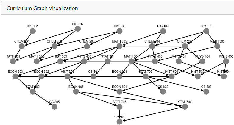
The application provides an intuitive interface that allows students, advisors, and administrators to dynamically interact with optimized degree plans. Users can select elective courses or modify program requirements, with real-time updates reflecting the impact of their choices. Immediate visual feedback is provided on critical metrics such as total credits per semester, average difficulty, and course cruciality values. Designed for scalability, the system efficiently processes large datasets involving hundreds of courses and complex hierarchical requirements. To enhance interpretability, the application incorporates multiple visualization tools that provide insights into curriculum structure, course dependencies, and degree plan optimization. The curriculum structure, including prerequisites and corequisites, is represented as a directed acyclic graph (DAG), where nodes correspond to courses annotated with their respective credits and pass rates, while directed edges illustrate prerequisite relationships. Figure 1 presents an example of this visualization.
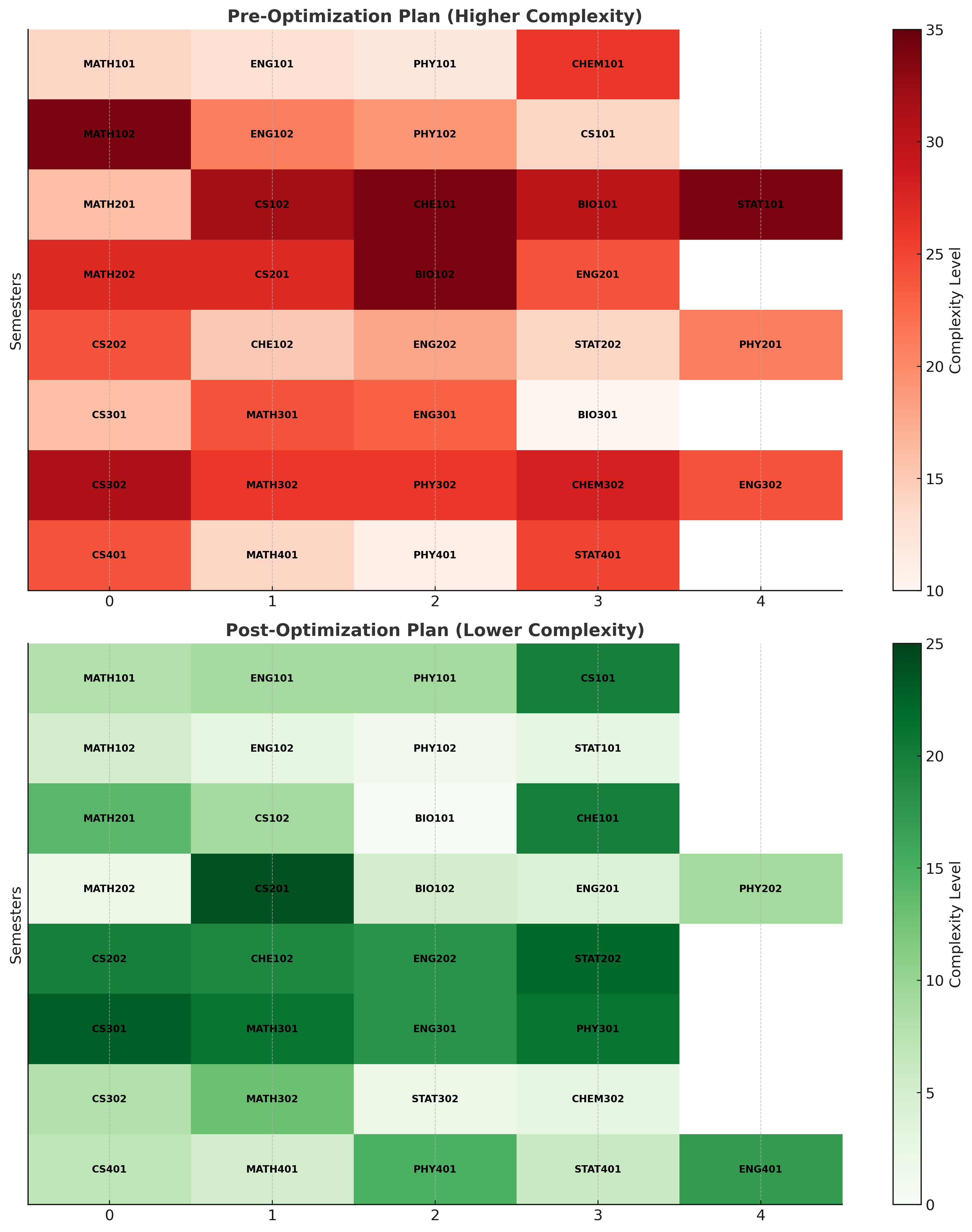
The impact of optimization is further highlighted through a direct graphical comparison of degree plans before and after optimization. Figure 2 showcases a pre-optimization degree plan, which exhibits higher curricular complexity, and the corresponding optimized plan, where complexity is reduced, and workload is more evenly distributed. This comparison visually reinforces the effectiveness of the proposed framework.
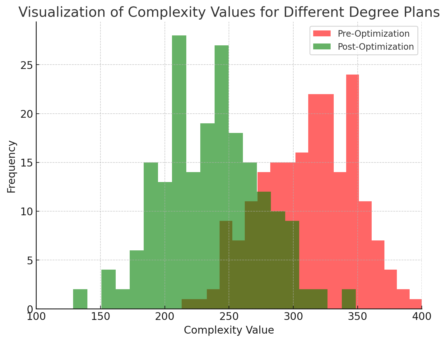
To assess the impact of curricular complexity on student outcomes, the application also visualizes complexity distributions across different degree plans. Figure 3 illustrates the distribution of complexity values, demonstrating how the optimization framework effectively minimizes unnecessary complexity while maintaining academic rigor.
6.2 Practical Applications and Future Enhancements
The application supports academic planning by providing personalized course selection guidance for students, data-driven recommendations for advisors, and curriculum analysis for administrators. It helps identify bottlenecks, optimize degree plans, and assess the impact of structural adjustments on student progression. Future enhancements will integrate Learning Management Systems (LMS) for real-time academic tracking, incorporate predictive analytics to estimate graduation probabilities, and offer customizable visualizations for tailored decision-making. By combining optimization techniques with interactive visualizations, the application transforms theoretical models into practical decision-support tools, enabling informed decisions that enhance student success.
7. RESULTS AND DISCUSSION
This section presents the outcomes of the proposed optimization framework, analyzing its effectiveness in satisfying academic requirements, minimizing curricular complexity, and ensuring balanced degree plans. Additionally, we discuss the broader implications of these results, comparing the framework with traditional methods and identifying areas for future enhancement. Studies in curricular analytics have consistently demonstrated a strong correlation between reduced curricular complexity and improved student success metrics, such as higher graduation rates and lower dropout rates [22, 6]. By optimizing course sequences to minimize structural bottlenecks, students experience smoother academic progression, reducing delays caused by prerequisite constraints. The degree plans analyzed in this study were generated using real student records from the University of New Mexico, ensuring practical relevance and applicability. The primary objective of the framework is to maximize satisfaction levels across all academic requirements. Table 3 summarizes the satisfaction levels for a sample academic program, demonstrating that core, elective, specialization, and capstone requirements are fully met. These results indicate the framework’s ability to accommodate diverse requirement structures, including shared and separate constraints.
| Requirement | Type | Satisfaction (\(y_r\)) |
|---|---|---|
| Core | Shared | 1.0 |
| Electives | Shared | 1.0 |
| Specialization | Separate | 1.0 |
| Capstone | Separate | 1.0 |
Beyond requirement satisfaction, minimizing curricular complexity is crucial for improving student progression and graduation rates [12]. Table 4 compares the complexity values of degree plans generated by the optimization framework with those produced by heuristic-based methods. The significant reduction in complexity highlights the framework’s ability to streamline course sequences, reducing bottlenecks and improving student outcomes.
| Method | Complexity Value |
|---|---|
| Proposed Optimization | 195 |
| Heuristic-Based Method | 220 |
| Baseline | 290 |
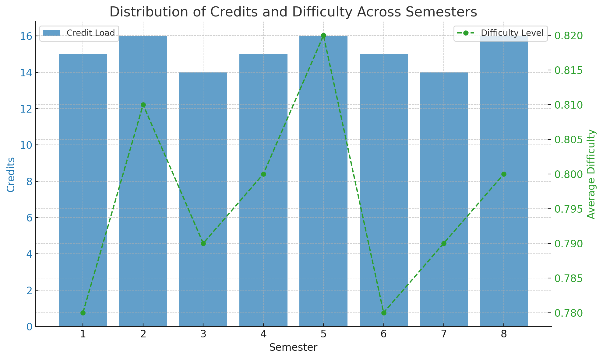
A well-structured degree plan must also maintain a balanced distribution of credit loads and difficulty across semesters. Figure 4 illustrates how the framework achieves an even allocation of credits and difficulty levels, preventing excessive student workload while ensuring steady academic progression.
The results underscore several key advantages of the proposed approach. By minimizing complexity and balancing course loads, the framework reduces barriers to timely graduation and supports student success [22, 6]. Additionally, its ability to model hierarchical constraints with precision enables informed decision-making for students, advisors, and administrators. Compared to traditional heuristic-based methods, the framework exhibits superior accuracy, scalability, and adaptability across different institutional contexts. However, certain challenges remain. The computational demands of solving large-scale MILP problems can be significant, particularly for highly complex curricula. The accuracy of the results depends on the availability of high-quality academic data, including pass rates and student performance metrics. Furthermore, while the framework offers a rigorous mathematical formulation, its complexity may pose interpretability challenges for non-technical stakeholders, necessitating effective visualization tools. Future work will focus on addressing these challenges and extending the framework’s capabilities. The integration of predictive analytics could enable dynamic adjustments to degree plans based on real-time academic data. Additionally, optimizing solver efficiency through parallel computing and advanced algorithms could further enhance performance. A user-centric approach to interface design and visualization will also improve accessibility, ensuring that students and advisors can effectively utilize the framework for decision-making. Overall, the results validate the effectiveness of the proposed optimization framework in satisfying academic requirements, minimizing curricular complexity, and balancing degree plans. By providing a structured, scalable, and data-driven approach to academic planning, this work contributes to improving student outcomes and institutional decision-making.
8. CONCLUSION AND FUTURE WORK
This paper presents an optimization framework for academic planning that maximizes requirement satisfaction, minimizes curricular complexity, and balances credit and difficulty distributions. By integrating hierarchical constraints and linearization techniques, the framework enhances computational efficiency for real-time degree planning. Validated with real-world data from the University of New Mexico, the framework effectively reduces curricular complexity, mitigates bottlenecks, and ensures balanced workloads, outperforming heuristic-based methods. Its structured, scalable approach supports personalized degree plans tailored to institutional and student needs. Challenges include addressing the computational demands of large-scale MILPs, ensuring data accuracy, and improving interpretability for non-technical users through better visualization tools. Future work will explore predictive models for dynamic curriculum adjustments, scalability improvements, and applications in other domains like workforce training. By combining theory with practical application, this framework provides a powerful data-driven tool to enhance academic planning and decision-making, ultimately fostering student success.
9. REFERENCES
- C. Adelman. The Toolbox Revisited: Paths to Degree Completion from High School Through College. U.S. Department of Education, Washington, DC, 2006.
- M. Backenköhler, F. Scherzinger, A. Singla, and V. Wolf. Data-driven approach towards a personalized curriculum. Proceedings of the 11th International Conference on Educational Data Mining, 2018.
- M. S. Bazaraa, J. J. Jarvis, and H. D. Sherali. Linear Programming and Network Flows. Wiley, 4th edition, 2009.
- D. Bertsimas and J. N. Tsitsiklis. Introduction to Linear Optimization. Athena Scientific, Belmont, MA, 1997.
- G. L. Heileman, C. T. Abdallah, A. Slim, and M. Hickman. Curricular analytics: A framework for quantifying the impact of curricular reforms and pedagogical innovations. CoRR, abs/1811.09676, 2018.
- S. Jones. The game changers: Strategies to boost college completion and close attainment gaps. Change: The Magazine of Higher Learning, 47(2):24–29, 2015.
- G. D. Kuh, J. Kinzie, J. H. Schuh, and E. J. Whitt. Student Success in College: Creating Conditions That Matter. Jossey-Bass, San Francisco, CA, 2005.
- G. L. Nemhauser and L. A. Wolsey. Integer and Combinatorial Optimization. John Wiley & Sons, 1988.
- M. L. Pinedo. Scheduling: Theory, Algorithms, and Systems. Springer, 6th edition, 2022.
- A. Slim. Curricular analytics in higher education. PhD thesis, The University of New Mexico, 2016.
- A. Slim, G. L. Heileman, C. T. Abdallah, A. Slim, and N. N. Sirhan. Restructuring curricular patterns using bayesian networks. In Proceedings of the International Conference on Educational Data Mining (EDM). Educational Data Mining (EDM), 2021.
- A. Slim, G. L. Heileman, M. Akbarsharifi, K. A. Manasil, and A. Slim. Causal inference networks: Unraveling the complex relationships between curriculum complexity, student characteristics, and performance in higher education. In 2024 ASEE Annual Conference & Exposition, 2024.
- A. Slim, G. L. Heileman, W. Al-Doroubi, and C. T. Abdallah. The impact of course enrollment sequences on student success. In 2016 IEEE 30th International Conference on Advanced Information Networking and Applications (AINA), pages 59–65. IEEE, 2016.
- A. Slim, G. L. Heileman, M. Hickman, and C. T. Abdallah. A geometric distributed probabilistic model to predict graduation rates. In 2017 IEEE SmartWorld, Ubiquitous Intelligence & Computing, Advanced & Trusted Computed, Scalable Computing & Communications, Cloud & Big Data Computing, Internet of People and Smart City Innovation (SmartWorld/SCALCOM/UIC/ATC/CBDCom/IOP/SCI), pages 1–8. IEEE, 2017.
- A. Slim, G. L. Heileman, J. Kozlick, and C. T. Abdallah. Employing markov networks on curriculum graphs to predict student performance. In 2014 13th International Conference on Machine Learning and Applications, pages 415–418. IEEE, 2014.
- A. Slim, G. L. Heileman, J. Kozlick, and C. T. Abdallah. Predicting student success based on prior performance. In 2014 IEEE Symposium on Computational Intelligence and Data Mining (CIDM), pages 410–415, 2014.
- A. Slim, G. L. Heileman, E. Lopez, H. A. Yusuf, and C. T. Abdallah. Crucial based curriculum balancing: A new model for curriculum balancing. In 2015 10th International Conference on Computer Science Education (ICCSE), pages 243–248, 2015.
- A. Slim, G. L. Heileman, H. A. Yusuf, Y. Zhang, A. Wasfi, M. Hayajneh, B. F. Mon, and A. Slim. Enhancing academic pathways: A data-driven approach to reducing curriculum complexity and improving graduation rates in higher education. In 2024 ASEE Annual Conference & Exposition, 2024.
- A. Slim, J. Kozlick, G. L. Heileman, and C. T. Abdallah. The complexity of university curricula according to course cruciality. In 2014 Eighth International Conference on Complex, Intelligent and Software Intensive Systems, pages 242–248. IEEE, 2014.
- A. Slim, J. Kozlick, G. L. Heileman, J. Wigdahl, and C. T. Abdallah. Network analysis of university courses. In Proceedings of the 23rd International Conference on World Wide Web, pages 713–718. ACM, 2014.
- A. Slim, H. A. Yusuf, N. Abbas, C. T. Abdallah, G. L. Heileman, and A. Slim. A markov decision processes modeling for curricular analytics. In 2021 20th IEEE International Conference on Machine Learning and Applications (ICMLA), pages 415–421. IEEE, 2021.
- V. Tinto. Leaving College: Rethinking the Causes and Cures of Student Attrition. University of Chicago Press, 2nd edition, 1994.
- S. Wasserman and K. Faust. Social Network Analysis: Methods and Applications. Cambridge University Press, Cambridge, UK, 1994.
- K. Xiang, X. Hu, M. Yu, and X. Wang. Exact and heuristic methods for a university course scheduling problem. Expert Systems with Applications, 248:123383, 2024.
© 2025 Copyright is held by the author(s). This work is distributed under the Creative Commons Attribution-NonCommercial-NoDerivatives 4.0 International (CC BY-NC-ND 4.0) license.