ABSTRACT
The aim of this paper is to provide tools to teachers for monitoring student work and understanding practices in order to help student and possibly adapt exercises in the future. In the context of an online programming learning platform, we propose to study the attempts (i.e., submitted programs) of the students for each exercise by using trajectory visualisation and clustering. To track the progress of students while performing exercises, we build numerical representations (embeddings) of their programs, generate the trajectories of these attempts (i.e., the sequence of their attempts) and provide an intuitive visualization of them. The advantage of these representations is to capture syntactic and semantic information that can be used to identify similar practices. In order to describe these practices, we perform a clustering of these attempts and generate a description of each cluster based on the common instructions of the underlying programs. By studying a student’s trajectory for an exercise, the teacher can detect if the student is in difficulty and help him. Our approach can also highlight atypical solutions such as alternative solutions or unwanted solutions. In the experiments, we study the impact of using embeddings to identify common practices on two real datasets. We also present a comparison of different dimension reduction methods (PCA, t-SNE, and PaCMAP) for the purpose of visualization. The experimental results show that code embeddings improve results compared to a classical approach, and that PCA and t-SNE are the most suitable for visualization.
Keywords
1. INTRODUCTION
In recent years, learning programming with online training platforms has increased significantly [2, 3]. The context can be online and massive or class-wide where students use the same platform during classes. Students submit their programs to the platform which returns any syntactic or functional errors based on test cases previously defined by the teacher. The use of data from these platforms makes it possible to develop tools for monitoring and helping to learn programming. There are a lot of works on the identification and prediction of student dropout [7, 16], the prediction of success (or failure) in exams [9], the management of hints [22] and the analysis of pedagogical feedbacks [27]. The aim of these tools is in particular to enable the teacher to be more responsive and effective in their interventions.
In this context, our work aims to provide teachers with tools for monitoring student work in order to help students as early as possible and thus avoid the accumulation of gaps, discouragement, and dropouts. We propose to follow students as they complete exercises by analyzing their submitted programs (i.e., attempts) for each exercise in term of trajectory visualization and clustering.
To analyze the attempts, it is necessary to consider the semantic aspect of the programs. To achieve this, we use representation learning [6], approaches known to build semantically rich representations of data. Initially developed to capture semantic aspects in text, they have been adapted to programs and other types of data. In our work, we consider more particularly two approaches that generate numerical vector representations of codes (embeddings) : CodeBERT [15] and code2aes2vec [10]. We use these representations to visualize similar practices and generate the attempts trajectories followed by students to solve an exercise. Three trajectory representations are compared. The first one is composed of the sequence of code embeddings representing each attempt submitted by the student. The second one is a sequence of scores indicating the cosine similarity between the submitted program and the teacher’s solution based on the code embeddings. The last one is a more classical approach [23] that represents the student’s trajectory as a sequence of scores based on the Levenshtein edit distance between the submitted program and the solution using the raw codes. In the experiments, we compare these representations on two real datasets. We also present a comparison of different dimensionality reduction methods (t-SNE, PCA, PaCMAP) [32] for visualization purposes.
In order to identify common practices of students to realize an exercise, we also perform a clustering of attempts, a clustering of trajectories and generate the description of each cluster based on the Abstract Syntax Trees (AST) of the programs. The first clustering enables to identify similar attempts. The keywords (”tokens”) common to programs in a cluster are used to describe the cluster. The second clustering of trajectories enables to highlight similar learning paths. Thus, our approach allows to visualize and describe the trajectories of students when solving an exercise, while taking into account the semantics of the underlying code.
By studying a student’s trajectory for an exercise, we can detect if the student is in difficulty so that the teacher can intervene to help him. We also highlight atypical solutions such as alternative solutions (correct solutions but not corresponding to the teacher’s) and unwanted solutions because they do not correspond to what the teacher asked. These detections can also lead the teacher to adapt an exercise (precision of statements, addition of test cases, etc.).
The rest of the paper is organized as follows. Section 2 discusses related work. We present our method to analyse students’ attempts in Section 3. We compare the proposed representations of attempts and the dimensionality reduction methods in Section 4. We conclude and give some perspectives in Section 5.
2. RELATED WORK
2.1 Analysis of Learning Trajectories
The analysis of learning trajectories, or knowledge tracing, is a growing area in AI for education, aiming to predict future student knowledge based on past performance to enable personalized interventions. In [1], the authors review various methods, including traditional Bayesian models and advanced deep learning techniques such as memory networks and attention-based models, to improve teaching strategy adaptation.
In [30], the authors introduce a visualization approach combining the t-SNE algorithm and Levenshtein distance. By calculating a distance matrix between each student’s attempt, they apply t-SNE to visualize students’ programming progress and categorize their activities at the class level. This interactive approach allows instructors to explore individual attempts and observe how students converge towards the expected final solution. They also developed a clustering algorithm based on Dynamic Time Warping (DTW) to identify common coding strategies among students. However, their approach doesn’t consider semantic aspects of codes.
In [23], similarity calculations and clustering techniques like k-means and the silhouette method are used to analyze learning trajectories based on the Damerau-Levenshtein distance between student attempts and instructor solutions. This method categorizes students into three groups: those who give up quickly, those who persist, and those who succeed efficiently. However, this approach focuses again on syntax, ignoring semantics, which limits the depth of trajectory analysis and does not offer detailed insights into the meaning of the clusters formed.
In [25], an initial approach for visualizing trajectories was proposed, followed by clustering attempts. It describes the students’ code status at different stages. This method suggests clustering the attempts. However, with this representation, it is difficult to group similar trajectories. In our work, we propose an additional visualization of the trajectories, alongside clustering and descriptions of the attempts, which allows for better clustering and characterization, ultimately leading to a deeper understanding of the data.
To the best of our knowledge, there are not many papers that take the same approach as ours, but there are still some that explore similar concepts. These works also emphasize the importance of visualizing and characterizing trajectories to gain a better understanding of student behaviors and performance. While our approach differs in certain aspects, particularly in the integration of representation learning, clustering and visualization for trajectory analysis, it shares common goals with these studies, focusing on improving the interpretability of learning patterns through advanced visual techniques.
2.2 Representation Learning from Codes
To effectively analyze learning trajectories, capturing the semantics of students’ programs is crucial. Recent studies have utilized representation learning to capture the semantics, adapting methods designed for text to work with code. These approaches aim to leverage the context in which ”words” (or ”tokens”) are used to create representations in the form of n-dimensional vectors (embeddings). This ability of embeddings to capture both semantic and syntactic aspects of code has been highlighted in [21]. In this work, the authors propose a framework for evaluating embeddings based on a 2D visualization of embeddings, a quantitative assessment of how well programs are grouped (e.g. programs are grouped by exercise), and an evaluation of the consistency of the embedding space using semantic and syntactic analogies.
One popular representation learning method is Doc2Vec [20], which extends this principle to learn document representations simultaneously. A more specialized approach, CodeBERT [15], adapts the BERT architecture, originally designed for text, to source code. BERT’s bidirectional framework enables it to capture contextual semantics effectively, making it highly effective for natural language processing tasks. CodeBERT modifies the tokenization method to handle source code.
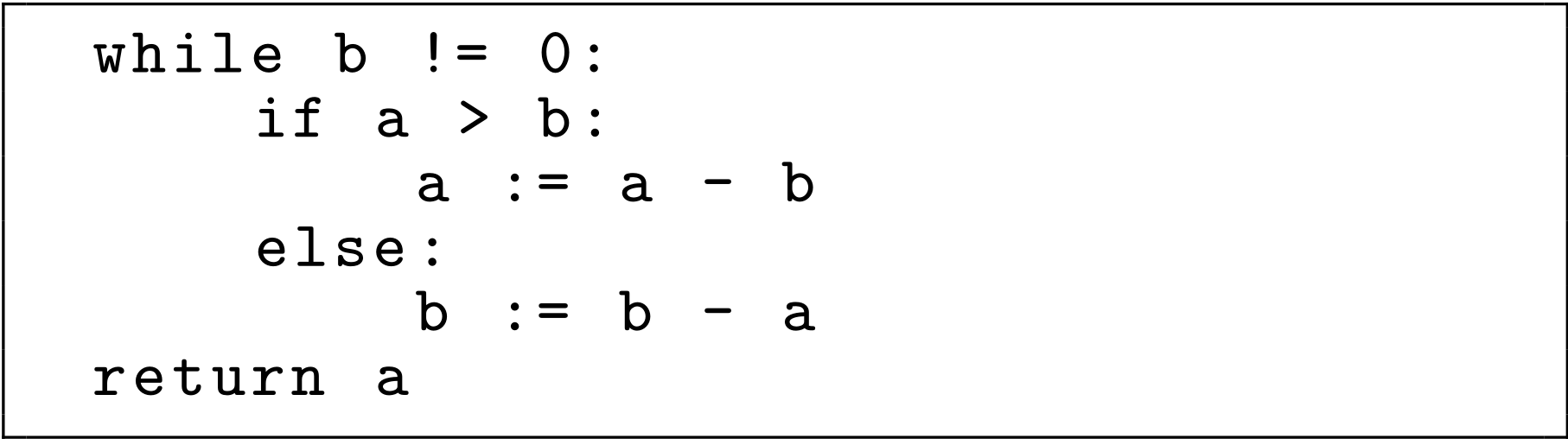
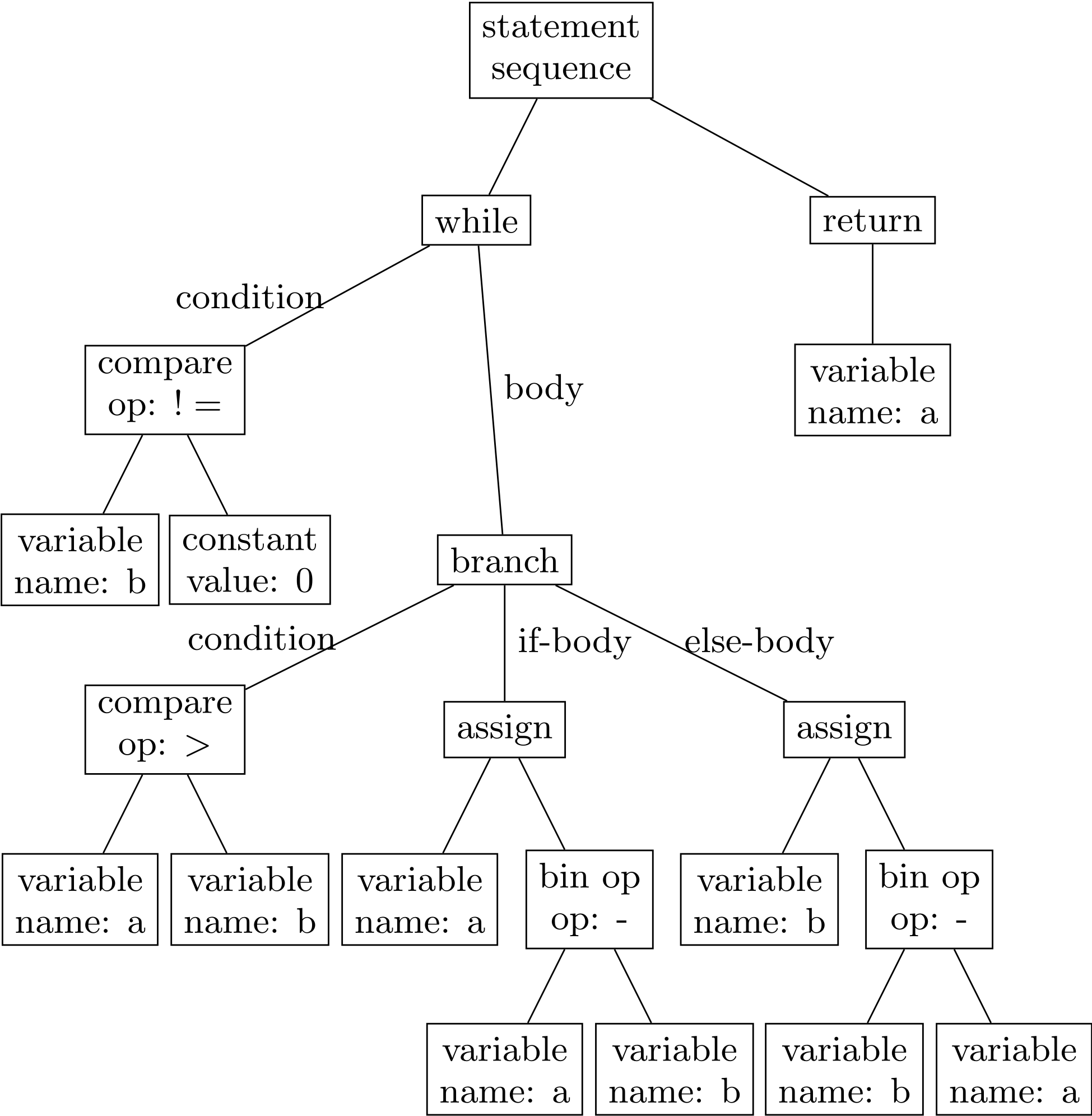
Another interesting model is code2aes2vec [10], which uses both the execution trace and the Abstract Syntax Tree (AST) of code to generate programs embeddings. Figure 2 illustrates a example of AST corresponding to the code presented in Figure 1. Based on the Doc2Vec architecture, it captures not only the syntactic aspects of code but also its logical structure, providing a richer and more meaningful vector representation.
Research on representation learning often employs dimensionality reduction algorithms to visualize high-dimensional embeddings (n-dimensional vectors) in a 2-dimensional space [32]. Common algorithms used include t-SNE , PaCMAP, and PCA.
PCA (Principal Component Analysis) [26] is a widely used linear technique that reduces dimensionality by identifying the principal components, or directions of maximum variance, in the data. While PCA is effective in retaining the most significant aspects of the data, it may struggle to capture complex nonlinear relationships compared to other methods. t-SNE (t-distributed Stochastic Neighbor Embedding) [31] is a nonlinear dimensionality reduction technique, primarily used for visualizing high-dimensional data. It aims to preserve local structures by placing similar points close together in the reduced space (usually 2 or 3 dimensions). t-SNE minimizes the divergence between probability distributions in high and low dimensions to achieve this. PaCMAP (Pairwise Controlled Manifold Approximation) [33] improves on t-SNE by balancing the preservation of both local and global structures. Unlike t-SNE, which focuses mainly on local relationships, PaCMAP optimizes the preservation of both short-range and long-range relationships, providing a better representation of the overall data structure while maintaining local coherence.
3. ANALYZING TRAJECTORIES OF STUDENTS’ ATTEMPTS
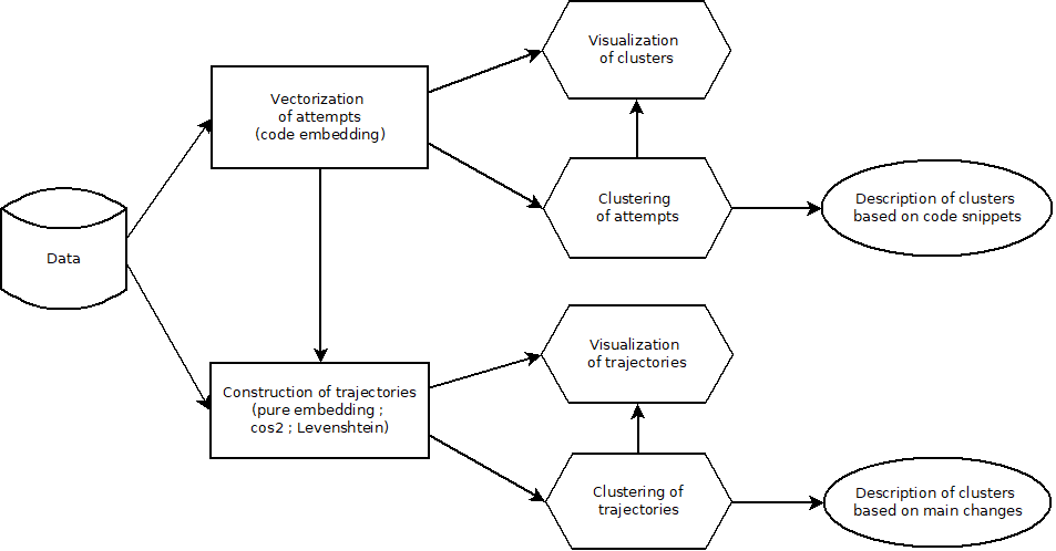
In this section, we present the proposed method to analyse students’ attempts based on program representation learning. The general overview of the method is shown in Figure 3. We compute various embeddings from the data using different models, such as code2aes2vec and CodeBERT. These embeddings enable us to construct trajectories using different methods. To gain deeper insights into student behavior and their learning paths, we propose multiple visualizations. Additionally, we apply clustering techniques at two levels. The first clustering groups coding attempts based on their embeddings, allowing us to develop an algorithm that categorizes attempts according to their coding patterns (e.g., a group predominantly using loops). The second clustering is applied to trajectories, grouping similar learning paths together. By leveraging both the clustering of attempts and trajectories, along with our proposed algorithm, we can effectively characterize students’ coding behaviors. The implementation and the datasets corresponding to this work are available on GitHub1.
3.1 Datasets
In this study, we utilized two real world datasets (cf. Table 1). The first dataset is derived from the use of an online platform for an introductory algorithm course at the University of New Caledonia [10]. This dataset, called NC5690, comprises 5,690 student attempts from 56 students across 66 Python programming exercises, including instructor solutions and unit tests. For our analysis, we used a smaller version of this dataset, called NC1014, containing 1,014 attempts across 8 exercises selected for their algorithmic diversity and balanced volume (with 100 to 150 programs per exercise). The second dataset, called Dublin, corresponds to student programs from the University of Dublin, from 2016 to 2019. While the original corpus contains nearly 600,000 Python and Bash programs, we used a subset that has been semi-automatically enriched with test cases (not initially provided). Each program has passed unit tests, which are small, automated checks that verify the correct functioning of individual pieces of code, such as functions or methods, in isolation. The resulted dataset includes 42,487 student attempts, 65 exercises, and 508 students.
| Dataset | NC1014 | NC5690 | Dublin |
|---|---|---|---|
| Nb. programs | 1,014 | 5,690 | 42,487 |
| Avg nb. test cases |
13.1 |
10.4 |
3.7 |
| \(\quad \)per program | |||
| Nb. correct programs | 189 | 1,304 | 19,961 |
| Nb. exercises | 8 | 66 | 65 |
3.2 Code Embedding
A code embedding specifically represents programming code as numerical vectors, aiming to encode its syntactic structure and semantic behavior. Examples include “tiny” models such that the code2aes2vec model, which learns embeddings from execution traces and abstract syntax trees (ASTs) in the training platform, and “big” models such that the CodeBERT model, pre-trained on large corpora of codes (GitHub) and contextual information. In this study, we use both code2aes2vec and CodeBERT to analyze and compare the representations of students’ programming attempts. By comparing the embeddings generated by these two methods, we aim to explore the differences and similarities in how they capture the key characteristics of students’ code.
3.2.1 Visualization of Attempts
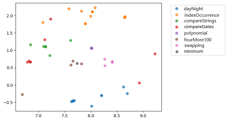
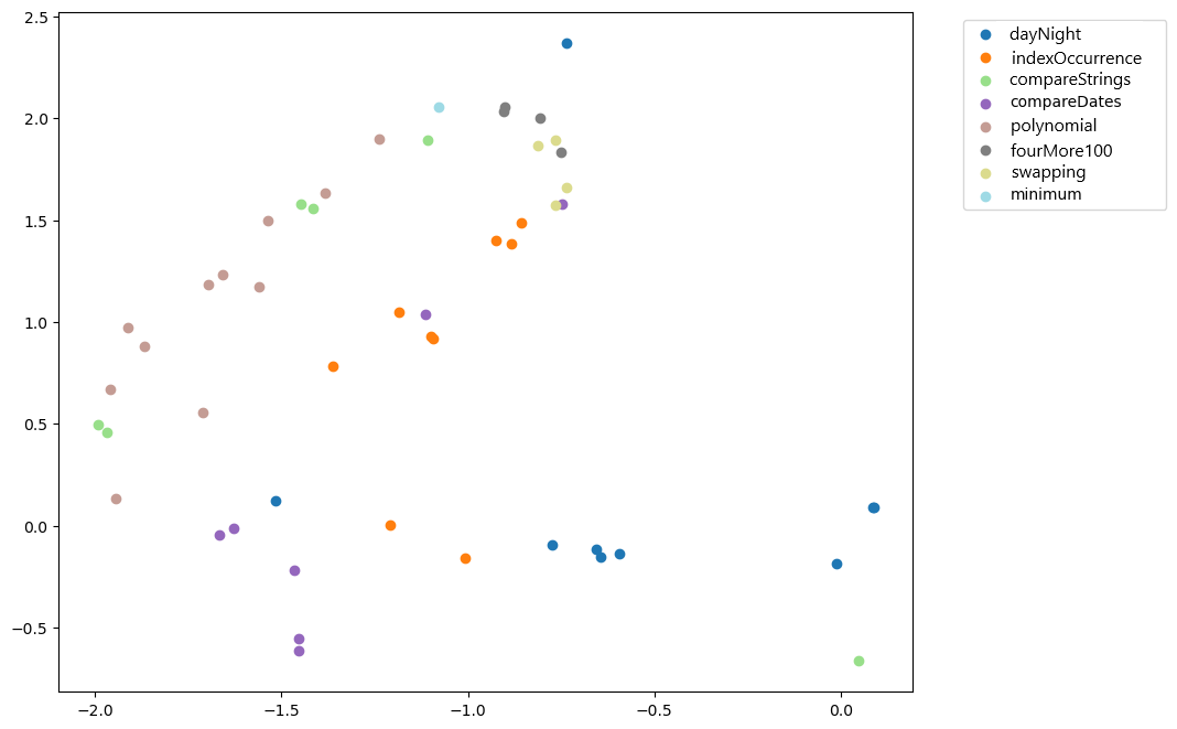
To visualize the embeddings, we use the t-SNE dimensionality reduction algorithm which project the 100-dimensional vectors as points in a 2D space. Even if these two dimensions are not directly explainable, this visualisation enables to estimates the distance of the students programs from each other, and their distance from the teacher’s solution. Since this representation space captures the syntax and semantics of programs, it is thus possible to see the different types of attempts. For example, Figures 4 and 5 present the result for code2aes2vec and CodeBERT, respectively. In Figure 4, we observe that the groups correspond to the different exercises, which suggests that the representation learning algorithm (code2aes2vec) has successfully captured the semantics of the programs despite relatively different syntaxes. In Figure 5, the results with CodeBERT are similar, but the clusters are less distinct. In particular, the clusters corresponding to the exercises are not as well-separated or defined as those produced by code2aes2vec, aligning with previous findings [10]. These observations emphasize the ability of both models to capture the syntax and semantics of code (as highlighted in the work of [21] discussed previously), validating their usefulness for analyzing students’ trajectories in detail.
3.2.2 Clustering of Attempts and Description of Clusters
We perform clustering of the embeddings in order to identify common practices among the programs submitted for the same exercise. To facilitate the use of this clustering by instructors, we also propose a method to describe these clusters based on their common instructions.
To perform the clustering, we use the Mean Shift algorithm [11], a variant of K-Means. Mean Shift has the advantage of not requiring the prior determination of the number of clusters, as it autonomously determines them. In addition, we obtained more exploitable results compared to other algorithms such as K-Means [17] or DBSCAN [14].
To describe a cluster, we exploit the AST of the programs associated with it. The keywords of the language (\(if\), \(while\), \(for\), etc.) are extracted, along with the operators associated with them (\(in\), \(not in\), \(=\), etc.). For example, if a program contains the statement if a >b, it will be characterized by (if, >. Thus, each program is characterized by a set of keywords corresponding to its statements. Then, each cluster is described by the common statements shared by all the programs it contains (by taking the intersection of the sets of statements). This description of programs can easily be extended to incorporate the frequency of occurrence of statements in the code. For example, a program with two for val in list loops could be represented as ((for, in), frequency: 2). This additional information provides the teacher with more details about the code submitted by the student.
By examining the common points between the attempts of a given cluster, it is possible to gain insights into the approach followed by a group of students to solve an exercise. Furthermore, it is common for a student to be associated with different clusters during their various attempts to solve the exercise. These changes in clusters are particularly interesting as they may reflect different ways of approaching the problem. Our approach allows us to capture this and describe these potential methodological shifts.
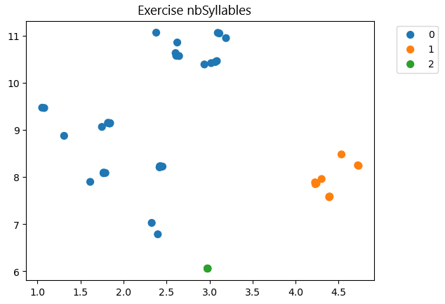
Figure 6 highlights three types of attempts for the ”number of syllables” exercise. The first group (orange, on the right) is described by the instructions (’for’, ’range’), (’augassign’, ’nonetype’), (’if’, ’notin’), (’assign’, ’list’) and (’assign’, ’subscript’). The second cluster (green, at the bottom) corresponds to the teacher’s solution and includes some instructions like (’for’, ’name’), (’return’, ’nonetype’), (’if’, ’eq’), (’assign’, ’binop’), (’assign’, ’constant’), (’if’, ’in’) and (’if’, ’nonetype’). The third cluster (blue, on the left) lacks distinctive features compared to the other groups. This suggests two possibilities for the students in the third group: either they solved the exercise without relying on the teacher’s specific approach, resulting in atypical solutions, or they are stuck at a certain level of understanding and failed to identify features present in other clusters, especially the teacher’s. Upon closer inspection, all students managed to get at least one correct answer, so these could be considered atypical solutions rather than indicative of a fundamental misunderstanding. In the next section, another type of visualization allows us to detect these atypical solutions more clearly.
3.3 Trajectories of Attempts
We generate the trajectories followed by students. A trajectory is defined as a sequence of attempts for a student on a particular exercise. We propose three strategies to construct trajectories of attempts. The first type of trajectory corresponds to a sequence of the embeddings of attempts (raw embedding method). The second one is a sequence of the cos\(^2\) distances between each attempt and the teacher’s solution using embeddings (cos\(^2\) method). The last one is a sequence of the Levenshtein distances applied to the attempts and the solution using raw code (Levenshtein method). In the construction of the trajectories, we focus on the order of the attempts rather than their timing. This decision is driven by the variability in submission dates, as students access the platform both in-person and remotely. If exercises had been completed within a more controlled time frame, submission dates could have been used for analysis, as seen in [23]. Our approach is generic and applicable to both sequences of embeddings and time series of embeddings.
3.3.1 Visualization of Attempts Trajectories
In order to guide teachers in analyzing students’ responses, we propose two types of visualizations of learning trajectories.
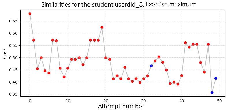
The first one is inspired by the visualization proposed in [23]. It highlights the similarity (using cos\(^2\) and Levenshtein methods) between the student’s attempt and the teacher’s solution, in the form of a time series (cf. Figure 7). The second one shows the position in the embedding space of the student’s attempt among all other attempts, along with the solution (cf. Figure 8).
Contrary to [23], the similarity used between the attempt and the solution is the cosine similarity between the two embedding vectors, rather than the Levenshtein distance between raw codes, which allows a better capture of both syntactic and semantic similarity. We also display the correct and incorrect attempts of the student in different colors (cf. Figure 7). In fact, several programs can be solutions to the same exercise, even if the teacher only records a single solution in the platform. These solutions from students are determined by the unit tests designed by the teacher, which are associated with each exercise. It is important to have this information because the student may present alternative solutions that are potentially far from the recorded solution. These could be atypical solutions, solutions based on poor practices, or incorrect solutions (if the unit tests were poorly designed). The teacher can thus detect these student solutions and study them in more detail. Let us note that this visualization can also be significantly adapted to highlight the distance from the closest solution, whether it is provided by the teacher or another student.
Figure 7 demonstrates the first visualization type, revealing variations in similarity with several programs close to the teacher’s solution. Notably, the student’s first attempt is closest to the teacher’s solution, but subsequent attempts deviate. Despite submitting three ”correct” programs that pass unit tests (the blue points), these solutions are far from the teacher’s solution, suggesting they may be atypical solutions or due to poorly designed tests. This visualization helps teachers analyze student progress and identify areas where further support is needed.
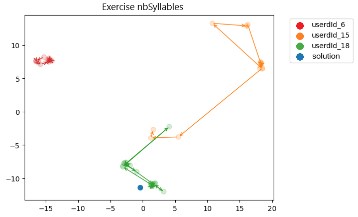
We propose a second visualization in the form of a 2D map. The goal is to provide an overview of the different attempts made for a given exercise. It displays the embeddings of the submitted programs (100-dimensional vectors in our experiments) as points in a 2-dimensional space. To achieve this, it is necessary to use dimensionality reduction techniques, such as t-SNE, PCA, or PaCMAP [32]. These points are then connected by arrows representing the successive submissions of a student to solve an exercise (i.e., the trajectory). This visualization allows the teacher to better understand how a student’s attempts evolve, how they may approach or diverge from different solutions, and how they position themselves (syntactically and semantically) in relation to the trajectories of other students. This methodical and multidimensional approach enables the proposal of personalized support strategies based on a deep understanding of the students’ learning trajectories.
Figure 8 illustrates the second visualization approach, showing the trajectories of three students for the ”number of syllables” exercise. The embedding trajectories highlight how students progress towards the teacher’s solution, and how a student changes his code over the course of attempts. Points that appear in darker colors represent successful attempts, while lighter-colored points indicate unsuccessful ones. Only Student 18 arrives at a correct program after being blocked between two relatively similar types of attempts. Conversely, Student 15 first proposes several programs that are relatively far from the teacher’s solution, then approaches the teacher’s solution, but does not reach it. Student 6 submits several incorrect programs (which are very similar) without progressing towards the solution. These trajectories can suggest that Student 15 and Student 6 are engaged in trial-and-error learning, emphasizing the need for targeted support to overcome final obstacles and achieve a success. Figure 8 offers strong pedagogical value, as it enables teachers to observe not only whether a student succeeds or fails, but also how they progress—or fail to progress—toward a solution. Rather than simply tracking a sequence of right or wrong answers, it reveals the direction of the student’s movement within the semantic space of the task. This allows for the identification of distinct learning profiles, such as students who experiment with various strategies, those who remain stuck, and those who quickly converge on the correct approach. Such insights are interesting for adapting teaching interventions, providing targeted support, and offering differentiated feedback. Moreover, the visualization facilitates a more refined diagnosis of learning difficulties; for instance, a student may appear close to the solution yet eventually stagnate, signaling a critical need for timely assistance—something that linear visualizations often fail to capture.
The first visualization shows the progression of student’s programs in relation to the teacher’s solution, focusing on similarity, while the second illustrates the positioning of student attempts within the overall space of all attempts for the exercise.
3.3.2 Clustering of Attempts Trajectories
After obtaining the different trajectories using the methods based on raw embeddings, cos\(^2\), and Levenshtein distance, clusterings are performed to observe similarities across the trajectories. Each clustering is done exercise by exercise, rather than globally. The used clustering algorithm is TimeSeriesKMeans [18]. Several algorithms have been tested (MeanShift [11], K-Means [17], DBSCAN [14], etc.), but they struggled to perform coherent grouping. Indeed, for an exercise with, for example, 15 trajectories, we have obtained more than ten different clusters, a problem that did not occur with TimeSeriesKMeans. Clustering trajectories helps group similar sequences of student attempts to understand how they succeed (or fail) in completing their exercises.
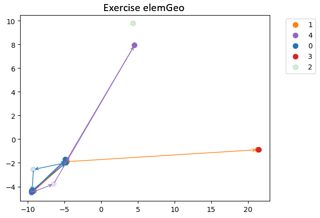
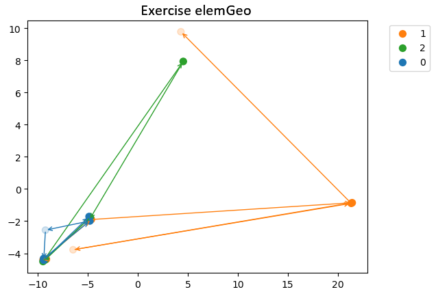
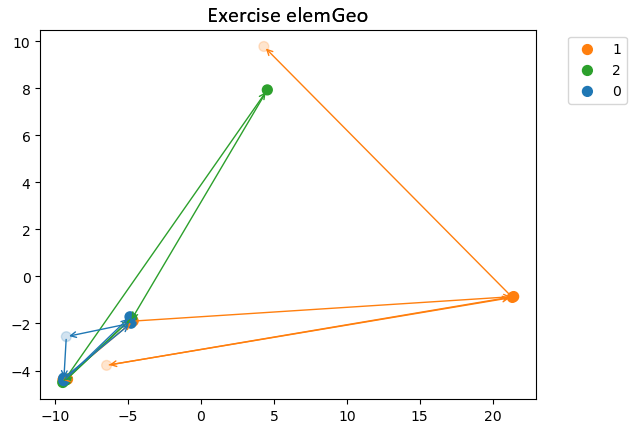
We performed clustering using the three methods (raw embeddings, cos\(^2\), and Levenshtein), as explained earlier. We can first observe that, for the method based on Levenshtein distance or cos\(^2\) similarity (cf. Figures 10 and 11), we find exactly the same clustering of trajectories. However, the clustering based on embeddings (cf. Figure 9) groups the trajectories differently from the other methods. The method based only on embeddings thus offers a different perspective compared to the other two methods. The key question is whether it produces a more meaningful and accurate clustering.
To address this, in the next section, we compare the methods to find which method yields the most relevant clustering.
4. EXPERIMENTAL COMPARISON
4.1 Comparison of the Attempts Representations
After performing the clusterings, exercise by exercise, using trajectories based on raw embeddings, cos\(^2\) similarity (based on embeddings), and Levenshtein distance (based on raw code), we then compare these methods to observe which one provides the most efficient grouping during the clustering. To do this, we use methods that calculate intra-cluster and extra-cluster distances, such as the silhouette score [28], the Davies-Bouldin index [12], and the Calinski-Harabasz index [8]. The silhouette score measures how similar an object is to its own cluster compared to other clusters. It ranges from -1 to +1, where a value closer to +1 indicates that the object is well-clustered, while a value closer to -1 suggests poor clustering. The Davies-Bouldin index evaluates the average similarity between each cluster and its most similar cluster, where lower values indicate better clustering results. Lastly, the Calinski-Harabasz score (also known as the Variance Ratio Criterion) measures the ratio of between-cluster dispersion to within-cluster dispersion. Higher values indicate more distinct clusters, with well-separated and compact clusters being preferred. We then compute the sum of their scores (the total silhouette score for all exercises, the total Davies-Bouldin index, and the total Calinski index). A higher value for silhouette and Calinski scores indicates better results, while a lower Davies-Bouldin index indicates better clustering performance.
For trajectories based on cos\(^2\) similarity and Levenshtein distance, no algorithm transformation is needed, as they are directly taken into account. For the method using the embeddings, we have reprogrammed these different algorithms to accept our embedding trajectories as input. Instead of considering a trajectory as a vector for the cos\(^2\) and Levenshtein methods (where we simply have a list of scores), we treat a trajectory as a matrix where each row corresponds to an embedding (a single attempt). We thus implement these different scoring methods using matrix distance for the embedding trajectories.
As a baseline, we also created random embeddings. For each existing embedding, we took the minimum and maximum values found. We then generated embeddings of length 100 with random values between the minimum and maximum. Afterward, we recomputed our methods using these new random embeddings. We labeled the method using random data as ”method random” in the tables presented the results.
| Method | Silouhette | Davies-Bouldin | Calinski |
|---|---|---|---|
| Embedding NC | 27.23 | 60.51 | 20,673.25 |
| cos\(^2\) NC | 2.21 | 127.56 | 417.15 |
| Leveinshtein NC | 24.73 | 37.17 | 1,521.52 |
| Embedding DB | 54.23 | 61.14 | 53,063.23 |
| cos\(^2\) DB | 64.91 | 27.72 | 22,800.53 |
| Leveinshtein DB | 61.61 | 33.37 | 70,965.99 |
| Embedding random | 20.74 | 112.13 | 562.97 |
| cos\(^2\) random | -0.75 | 160.32 | 55.74 |
| Leveinshtein random | 2.61 | 153.21 | 236.74 |
Each column in Table 2 represents a metric used to evaluate the quality of the clustering. We can see in this table with the first dataset (NC5690), the embeddings method outperformed the other two methods, except for the Davies-Bouldin index. This indicates that clustering using embedding trajectories generally results in better groupings than using raw code (i.e., Levenshtein). When testing on a second dataset (10% of the Dublin dataset in Table 2), the cos\(^2\)-based method, which also incorporates embeddings, produced the best results, rather than raw embeddings. We can observe that embeddings (pur embedding method or cos\(^2\) method) provide a significant contribution and differ from raw code in their impact. This distinction becomes clear when analyzing the results, as they demonstrate that the use of embeddings leads to the formation of higher-quality clusters. This improvement is particularly noticeable when evaluating the different clustering scores presented, which indicate a more structured and relevant grouping of data compared to using raw code alone.
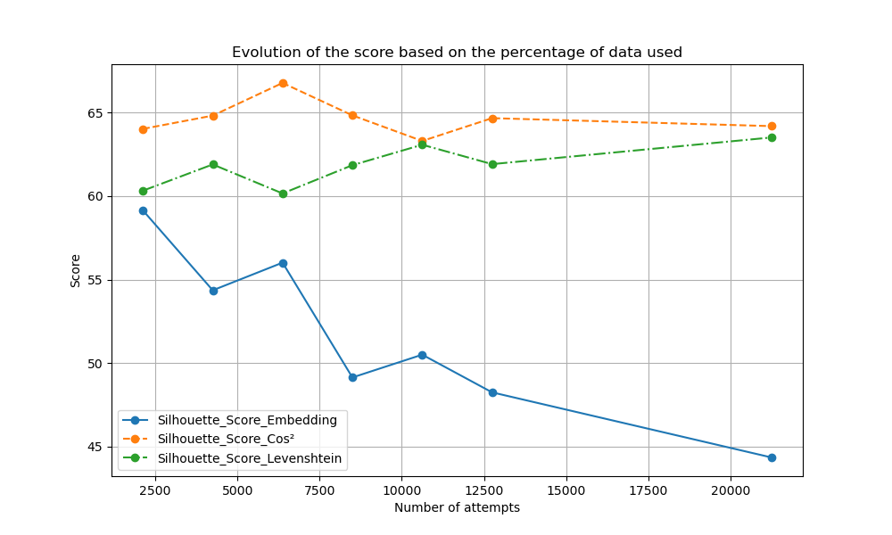

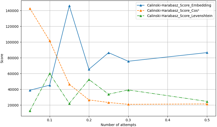
We also examined how clustering scores evolved based on the number of attempts in the Dublin dataset (in Figures 13, 14 and 12). For the embeddings method, significant variation in the Calinski-Harabasz index suggested that the addition of new attempts might either introduce noise or improve clustering by logically continuing distant attempts. The Davies-Bouldin index increased while the Silhouette score decreased as the dataset grew, indicating a decline in clustering quality.
For the cos\(^2\) method, the Calinski-Harabasz index dropped, the Silhouette score remained stable, and the Davies-Bouldin index sharply increased, suggesting a degradation in clustering. The Levenshtein method showed similar trends to the embeddings method, with stable Silhouette scores and a modest increase in the Davies-Bouldin index. This degradation of the Calinski-Harabasz and Davies-Bouldin scores is due to their higher sensitivity to intra-cluster variability. As more data is added, the clusters become less compact and more dispersed, increasing intra-cluster heterogeneity. This results in a decrease in the Calinski-Harabasz index and an increase in the Davies-Bouldin index, indicating a decline in clustering quality. The additional data points introduce greater variability within clusters, making them less well-defined while also reducing the overall separation between them.
Overall, embedding-based methods (raw embeddings and cos\(^2\)) outperformed the Levenshtein method in Silhouette and Calinski scores. However, the Levenshtein method remained superior for the Davies-Bouldin index, particularly as the dataset size increased. Despite discrepancies caused by multi-function attempts in the Dublin dataset, embedding based methods consistently delivered superior results, confirming that embeddings offer more valuable information than raw code alone.
4.2 Comparison of the Dimensionality Reduction Algorithms
In this section, we study the visualization of high-dimensional embeddings in two dimensions using three dimensionality reduction algorithms: t-SNE, PCA, and PaCMAP. The main challenge is the loss of information during reduction, which is addressed by comparing the algorithms based on their ability to minimize this loss.
The first method groups embeddings by exercise and calculates the similarity between each embedding and all others within the same exercise, for both the original (before using dimensionality reduction algorithms) and reduced embeddings (after using dimensionality reduction algorithms). The absolute difference in similarity scores is then summed to generate an overall error score for each algorithm.
The second method (denoted ”Permutation” in Table 3) considers the order of the neighbors of an attempt, rather than their distance. For each exercise, it assigns random indices to the different attempts. For a given attempt (an embedding), it lists the closest attempts in the original embedding space using the Euclidean distance. It then does the same in the embedding space reduced by the different visualization approaches. Then, it calculates the number of permutations needed to go from the second sequence to the first. This number represents the number of changes to be made to correct the neighborhood of the attempt so that it matches that of the original embedding space. Thus, fewer permutations indicate better performance. This method will do the same for all attempts and sum the number of permutations. For example, if for Attempt 7, the closest attempts in the embedding space are the attempts 7, 1, 8, 9, 6, and those in the visualization space (embedding space reduced in 2 dimensions) are the attempts 7, 8, 1, 9, 6, then only one permutation would be needed to align the two sequences.
Both methods aim to identify the algorithm that best preserves the original data structure while reducing its dimensions, with the least information loss being the key measure of effectiveness. In summary, the lower the value is, the less information is lost during the application of the dimensionality reduction algorithm.
| Method | t-SNE | PCA | PaCMAP |
|---|---|---|---|
| Real_embedding_NC | 3,299 | 3,130 | 3,458 |
| Real_embedding_DB | 42,480 | 39,050 | 46,024 |
| Permutation_NC | 15,949 | 15,974 | 16,176 |
| Permutation_DB | 215,483 | 215,535 | 216,109 |
Table 3 presents the results. For the first method, PaCMAP achieves the highest score, significantly underperforming the other two methods, which show similar results. This suggests that PaCMAP might lose substantial information during dimensionality reduction. Since PCA achieved the lowest score, it suggests that it is the algorithm that lost the least amount of information. The second method (permutation) shows the same result for PaCMAP, being the one of the three that loses the most information. However, similar results are shown for PCA and t-SNE, although t-SNE performs slightly better in this case.
It is difficult to conclude that PCA is better than t-SNE, or vice versa, but based on the results from the first method, where PCA achieves better scores, we may later favor PCA as the dimensionality reduction algorithm. Further investigation could be conducted on the results obtained from PCA to gain a deeper understanding of its performance.
5. CONCLUSION
In this paper, we analyze programs submitted by students on an online learning platform, by considering the sequences of attempts as trajectories. We study how representation learning and dimensionality reduction approaches can help teachers in visualizing and understanding students’ learning practices.
More precisely, we have considered three types of representations for attempts: the submitted program embedding (i.e., a vector representation), a score corresponding to the cosine similarity between the submitted program and the teacher’s solution using code embeddings, and a score indicating the similarity with the teacher’s solution using raw codes and the Levenshtein distance. Based on these representations, we have performed clustering of attempts and trajectories in order to capture similar practices between the students. The experiments on two real datasets have shown that using embeddings (”raw embeddings” or ”\(cos^2\)-based”) give the best results.
For trajectory analysis, we also have proposed several types of visualization allowing the teacher to follow the progress of a student when carrying out an exercise. These visualizations can allow the teacher to detect if a student is in difficulty (like a blocked situation) so that he can help him. They can also highlight atypical solutions such as alternative solutions (correct solutions but not corresponding to the teacher’s solution) and unwanted solutions because they do not correspond to what the teacher asked. These atypical solutions can lead the teacher to refine an exercise (precision of the statements, addition of test cases, ...). On the studied datasets, we have also compared several dimension reduction algorithms (PCA, t-SNE, and PaCMAP) for visualization purposes. We have observed that PCA and t-SNE are the most suitable.
These visualizations lay the groundwork for developing tools that support pedagogical analysis. Eventually, such visualizations could be integrated into a teacher dashboard, offering features such as individual or group trajectory views, automatic indicators of stagnation or atypical solutions, and suggestions for grouping students based on their strategies or error types. The aim is to assess the readability and usability of these visualizations for teachers who are not experts in visual analytics, to evaluate their impact on teaching practices and student learning, and to refine the visualizations based on user feedback.
A major perspective of this work is to provide teachers explainable embeddings’ dimensions, and trajectories. Explainability is an important topic actually in AI [5, 19, 13, 4] since current neural network based approaches are mainly black boxes. For this, an idea is to adapt the works of [24, 29] to provide explainable dimensions by generating non-negative sparse embeddings. Using such approach, we could propose an interactive visualization where the two dimensions of analysis displayed on the graph would be chosen by the teacher according to the aspects he wishes to analyze. We will also work on adapting time series classification algorithms to detect students on ”wrong” trajectories early, and integrating data on the student profile in the analysis. We will create other datasets in order to extend the field of application, for example, to other programming languages. We will integrate our propositions into a online learning platform to provide decision support tools for teachers and to enable real-time interventions.
6. REFERENCES
- G. Abdelrahman, Q. Wang, and B. Nunes. Knowledge tracing: A survey. ACM Computing Surveys, 55:1–36, 2022.
- R. Albashaireh and H. Ming. A survey of online learning platforms with initial investigation of situation-awareness to facilitate programming education. In 11th Int. Conf. on Computational Science and Computational Intelligence, pages 631–637, Las Vegas, NV, USA, December 2018.
- N. Alhammad, A. B. Yusof, F. Awae, H. Abuhassna, B. I. Edwards, and M. A. B. M. Adnan. E-Learning Platform Effectiveness: Theory Integration, Educational Context, Recommendation, and Future Agenda: A Systematic Literature Review, pages 101–118. Springer, Singapore, 2024.
- S. Ali, T. Abuhmed, S. El-Sappagh, K. Muhammad, J. M. Alonso-Moral, R. Confalonieri, R. Guidotti, J. Del Ser, N. Díaz-Rodríguez, and F. Herrera. Explainable artificial intelligence (xai): What we know and what is left to attain trustworthy artificial intelligence. Information fusion, 99:101805, 2023.
- A. B. Arrieta, N. Díaz-Rodríguez, J. Del Ser, A. Bennetot, S. Tabik, A. Barbado, S. García, S. Gil-López, D. Molina, R. Benjamins, et al. Explainable artificial intelligence (xai): Concepts, taxonomies, opportunities and challenges toward responsible ai. Information fusion, 58:82–115, 2020.
- Y. Bengio, A. Courville, and P. Vincent. Representation learning: A review and new perspectives. IEEE transactions on pattern analysis and machine intelligence, 35(8):1798–1828, 2013.
- P. Buñay Guisñan, J. A. Lara, A. Cano, R. Cerezo, and C. Romero. Easing the prediction of student dropout for everyone integrating automl and explainable artificial intelligence. In 17th Int. Conf. on Educational Data Mining, page 857–861, Atlanta, Georgia, USA, July 2024.
- T. Caliński and J. Harabasz. A dendrite method for cluster analysis. Communications in Statistics-theory and Methods, 3(1):1–27, 1974.
- H. Chen and P. Ward. Clustering students using pre-midterm behaviour data and predict their exam performance. In 15th Int. Conf. on Educational Data Mining, page 689–694, Durham, UK, July 2022.
- G. Cleuziou and F. Flouvat. Learning student program embeddings using abstract execution traces. In 14th Int. Conf. on Educational Data Mining, pages 252–262, Paris, France, June 2021.
- D. Comaniciu and P. Meer. Mean shift: a robust approach toward feature space analysis. IEEE Transactions on Pattern Analysis and Machine Intelligence, 24(5):603–619, 2002.
- D. L. Davies and D. W. Bouldin. A cluster separation measure. IEEE Transactions on Pattern Analysis and Machine Intelligence, 1(2):224–227, 1979.
- W. Ding, M. Abdel-Basset, H. Hawash, and A. M. Ali. Explainability of artificial intelligence methods, applications and challenges: A comprehensive survey. Information Sciences, 615:238–292, 2022.
- M. Ester, H.-P. Kriegel, J. Sander, X. Xu, et al. A density-based algorithm for discovering clusters in large spatial databases with noise. In 2nd Int. Conf. on Knowledge Discovery and Data Mining, pages 226–231, Portland, Oregon, USA, 1996.
- Z. Feng, D. Guo, D. Tang, N. Duan, X. Feng, M. Gong, L. Shou, B. Qin, T. Liu, D. Jiang, and M. Zhou. CodeBERT: A pre-trained model for programming and natural languages. In Findings of the Association for Computational Linguistics (EMNLP), pages 1536–1547. Association for Computational Linguistics, 2020.
- O. Goren, L. Cohen, and A. Rubinstein. Early prediction of student dropout in higher education using machine learning models. In 17th Int. Conf. on Educational Data Mining, page 349–359, Atlanta, Georgia, USA, July 2024.
- J. A. Hartigan, M. A. Wong, et al. A k-means clustering algorithm. Applied statistics, 28(1):100–108, 1979.
- X. Huang, Y. Ye, L. Xiong, R. Y. Lau, N. Jiang, and S. Wang. Time series k-means: A new k-means type smooth subspace clustering for time series data. Information Sciences, 367:1–13, 2016.
- M. Langer, D. Oster, T. Speith, H. Hermanns, L. Kästner, E. Schmidt, A. Sesing, and K. Baum. What do we want from explainable artificial intelligence (xai)?–a stakeholder perspective on xai and a conceptual model guiding interdisciplinary xai research. Artificial intelligence, 296:103473, 2021.
- Q. Le and T. Mikolov. Distributed representations of sentences and documents. In 31st Int. Conf. on Machine Learning, page 1188––1196, Beijing, China, June 2014.
- T. Martinet, G. Cleuziou, M. Exbrayat, and F. Flouvat. From document to program embeddings: can distributional hypothesis really be used on programming languages? In ECAI 2024, pages 2138–2145. IOS Press, 2024.
- J. McBroom, I. Koprinska, and K. Yacef. A survey of automated programming hint generation: The hints framework. ACM Computing Surveys, 54(8):1–7, 2021.
- F. Morshed Fahid, X. Tian, A. Emerson, J. B. Wiggins, D. Bounajim, A. Smith, E. Wiebe, B. Mott, K. Elizabeth Boyer, and J. Lester. Progression trajectory-based student modeling for novice block-based programming. In 29th ACM Conf. on User Modeling, Adaptation and Personalization, pages 189–200, Utrecht, the Netherlands, June 2021.
- B. Murphy, P. P. Talukdar, and T. Mitchell. Learning effective and interpretable semantic models using non-negative sparse embedding. In International Conference on Computational Linguistics (COLING 2012), Mumbai, India, pages 1933–1949. Association for Computational Linguistics, 2012.
- B. Paassen, J. McBroom, B. Jeffries, I. Koprinska, K. Yacef, et al. Mapping python programs to vectors using recursive neural encodings. Journal of Educational Data Mining, 13(3):1–35, 2021.
- K. Pearson. Liii. on lines and planes of closest fit to systems of points in space. The London, Edinburgh, and Dublin philosophical magazine and journal of science, 2(11):559–572, 1901.
- G. Raubenheimer, B. Jeffries, and K. Yacef. Toward empirical analysis of pedagogical feedback in computer programming learning environments. In the 23rd Australasian Computing Education Conference, pages 189–195, Virtual, SA, Australia, 2021.
- P. J. Rousseeuw. Silhouettes: a graphical aid to the interpretation and validation of cluster analysis. Journal of computational and applied mathematics, 20:53–65, 1987.
- A. Subramanian, D. Pruthi, H. Jhamtani, T. Berg-Kirkpatrick, and E. Hovy. Spine: Sparse interpretable neural embeddings. Proceedings of the AAAI Conference on Artificial Intelligence, 32(1):4921–4928, 2018.
- Y. Taniguchi, T. Minematsu, F. Okubo, and A. Shimada. Visualizing source-code evolution for understanding class-wide programming processes. Sustainability, 14, 8084, 2022.
- L. Van der Maaten and G. Hinton. Visualizing data using t-sne. Journal of Machine Learning Research, 9(86):2579–2605, 2008.
- Y. Wang, H. Huang, C. Rudin, and Y. Shaposhnik. Understanding how dimension reduction tools work: an empirical approach to deciphering t-sne, umap, trimap, and pacmap for data visualization. Journal of Machine Learning Research, 22(201):1–73, 2021.
- Y. Wang, H. Huang, C. Rudin, and Y. Shaposhnik. Understanding how dimension reduction tools work: An empirical approach to deciphering t-sne, umap, trimap, and pacmap for data visualization. Journal of Machine Learning Research, 22(201):1–73, 2021.
© 2025 Copyright is held by the author(s). This work is distributed under the Creative Commons Attribution-NonCommercial-NoDerivatives 4.0 International (CC BY-NC-ND 4.0) license.