ABSTRACT

We propose an innovative, effective, and data-agnostic method to train a deep-neural network model with an extremely small training dataset, called VELR (Voting-based Ensemble Learning with Rejection). In educational research and practice, providing valid labels for a sufficient amount of data to be used for supervised learning can be very costly and often impractical. The shortage of training data often results in deep neural networks being overfitting. There are many methods to avoid overfitting such as data augmentation and regularization. Though, data augmentation is considerably data dependent and does not usually work well for natural language processing tasks. Moreover, regularization is often quite task specific and costly. To address this issue, we propose an ensemble of overfitting models with uncertainty-based rejection. We hypothesize that misclassification can be identified by estimating the distribution of the class-posterior probability P(y|x) as a random variable. The proposed VELR method is data independent, and it does not require changes to the model structure or the re-training of the model. Empirical studies demonstrated that VELR achieved classification accuracy of 0.7 with only 200 samples per class on the CIFAR-10 dataset, but 75% of input samples were rejected. VELR was also applied to a question generation task using a BERT language model with only 350 training data points, which resulted in generating questions that are indistinguishable from human-generated questions. The paper concludes that VELR has potential applications to a broad range of real-world problems where misclassification is very costly, which is quite common in the educational domain.

Keywords

INTRODUCTION

When applying a deep-neural network to real-world classification tasks, it is sometimes the case that only a very small amount of labeled data is available for training a model. When a deep neural-network (DNN) model is trained with a small amount of data, the model often overfits to the training data due to over-parameterization. We call such a problematically small amount of data the extremely low data regime [36].

Regularization is a widely used technique to prevent the model from overfitting. However, it requires the hyperparameters to be fine-tuned a priori, and the model must be retrained each time the hyperparameters are changed.

Another commonly used technique that is known to be an effective solution to the overfitting problem is semi-supervised learning, which utilizes unlabeled data in conjunction with labeled data for training [30, 33]. In recent years, data augmentation using Generative Adversarial Networks (GAN) has been actively studied to synthetically inflate data, significantly improving the performance of semi-supervised learning [4, 6, 10, 19]. However, there are situations where only a small amount of labeled data is available and data augmentation is not a suitable option. Text analysis in natural language processing is an example of one such data-augmentation incompatible task.

Although some research has demonstrated that DNN models can generalize well with extremely small data regimes, the performance is still lower than that of when an abundant amount of data is available [26, 32]. Low performance due to overfitting is a serious problem, especially when the model is used for real-world tasks where misclassification can be very costly and even unethical such as medical diagnoses or educational interventions. To further expand the application of DNN to real-word tasks, it is therefore critical to develop a technique that can overcome the overfitting problem with extremely low data regimes.

In this study, we propose a rigorous ensemble technique for estimating class-posterior probabilities based on a collection of overfitting models. Our proposed method does not use any regularization techniques or generative models for data augmentation to avoid overfitting. Instead of preventing overfitting while training models, we propose to identify unreliable classification using a soft voting ensemble method based on the distribution of the estimated class-posterior probability P(y|x) among the collection of overfitting models.

In other words, we aggregate the class-posterior probabilities P(y|x) from multiple isomorphic models (aka soft voting) instead of aggregating the class prediction y (aka hard voting) [37]. We treat P(y|x) as a random variable while considering a predicted class-posterior probability from each model as an observation to estimate the distribution of this random variable.

An unreliable classification will be rejected to reduce the risk of giving wrong predictions. We shall call our proposed method Voting-based Ensemble Learning with Rejection (VELR).

With a lack of theoretical work in the design of a voting technique, we explored two soft-voting methods: min-majority voting and uniform voting. The min-majority voting estimates Gaussian Mixture Models and takes the minimum probability in a majority cluster, whereas uniform voting sums the probabilities with a uniform weight. Although uniform voting itself is not novel, voting among overfitting models due to the extremely low data regime has not been studied, as far as we are aware.

In addition, it is not clear in the current literature how classification with rejection works in conjunction with voting over an ensemble of overfitting models. We demonstrated that classification with rejection with voting shows a better performance than that with a single model when only an extremely low data regime is available.

To validate VELR, we conducted evaluation studies on two tasks: (1) image classification on a commonly used bench-mark dataset and (2) pedagogical question generation for online courseware engineering. The results showed that voting-based ensemble learning with rejection was able to identify incorrect predictions and accuracy of classification increased significantly by rejecting those predictions.

Our contributions are as follows: (1) We propose voting-based ensemble learning with rejection, VELR, a practical and data-agnostic solution for training deep-neural network models with extremely small datasets that would otherwise be overfit to the training data. (2) We show that a combination of soft voting among overfitting models and rejection can significantly increase performance of a model that relies on estimation of a class-posterior probability. (3) We demonstrated that VELR is data agonistic through two empirical studies—image and text analyses. (4) The code and data used for the current study have been open sourced^[1].

VELR: voting-based ensemble learning with rejection

Training the Base Models

VELR applies to any deep-neural network model that outputs normalized posterior probability (or certainty), P(y|x) = [0, 1], which means that when multiple certainties are output (e.g., multi-label classification), the sum of P(y_i|x) are 1 across all outputs. In the current paper, we assume multiple certainties are output, but it sshould be clear that the same logic applies to models with a single certainty, e.g., a binary classification.

Suppose we have an input x ∈ X in a multi-dimensional space and class labels Y = {y₁, y₂, ..., y_C}. In general, to train a classification model is to optimize a set of certainties P(y_iÎY|x) in a training dataset.

When trained with an extremely low data regime, the model will unavoidably overfit. We therefore propose to create a collection of models that are independently trained using the same deep-neural network structure, the same training dataset, and the same hyperparameter settings. It is only that the random initial weights are different. Accordingly, a set of certainty P^m(y_iÎY|x) for a sample x are computed, each independently by an individual model m (m = 1, …, M) as depicted in Figure 1. The question is how to make a consensus among multiple certainties. The next section describes a voting technique to compute the consensus certainty P*(y_iÎY|x).

Voting on Estimated Certainty Distribution

An essential problem of ensemble learning is to determine which posterior probability, among a collection of competing ones, should be taken. In the current literature, one approach takes model as the unit of analysis—i.e., individual models make a prediction based on their own posterior probabilities and then a majority vote is taken from the set of those predictions, aka hard voting [2].

VELR takes a different approach, where certainty is used as the unit of analysis. Namely, for each class y_i Î Y, VELR makes an ensemble decision about the posterior probability P*(y_iÎY|x) based on a set of certainties, P^m(y_iÎY|x), m = 1, …, M, as shown in Figure 1. In the current literature, this approach is called soft voting [37]. In the rest of this paper, we call P*(y_iÎY|x) as the consensus certainty^[2].

We explored two different methods for voting: min-majority voting and uniform voting, as shown in the following subsections. Our basic hypothesis is that voting decisions should be made based on the distribution of the certainty P(y_i|x) per class y_i among the M models. Therefore, we define a random variable $v^{y_{i}} = \{ v_{\mathbf{x},m}^{y_{i}} = P^{m}\left( y_{i} \middle| \mathbf{x} \right);\ m = 1,\ldots,M\}$ for each sample x and class y_i. We hypothesize that the decision of classification should be made based on voting among $v$’s.

Min-majority voting

For the min-majority voting, we assume that $v^{y_{i}}$ follows the Gaussian Mixture Model (GMM) defined as:

$$P\left( v^{y_{i}} \right) = \sum_{k = 1}^{K}{\pi_{k}\mathcal{N(}v^{y_{i}}|\mu_{k},\ \sigma_{k})}$$

$$\Sigma_{k = 1}^{K}\pi_{k} = 1,$$

$$\mathcal{\ \ N}\left( v^{y_{i}} \middle| \mu_{k},\ \sigma_{k} \right)\ \text{:\ }\text{Gaussian}\text{\ }\text{Density\ function}\text{\ }$$

$$\text{\ }K:Number\ of\ clusters$$

As Salman and Liu [25] analyzed, when models are overfitting, the probability distribution of the random variable $v$ tends to skew towards 0 and 1. We therefore assume K = 2 in the current implementation of VELR.

For each sample x, the estimation of π, μ, and σ is done by the EM algorithm [7] over the random variable $v$ as mentioned above.

Once the density functions are estimated, VELR finds the majority cluster that indicates the most dominant distribution of $v^{y_{i}}$ as defined below:

$$k_{majority} = argmax_{k \in K}\ \pi_{k}$$

Let $v_{\mathbf{x},m}^{y_{i}}$ be an observation of $v^{y_{i}},\$which is $P^{m}\left( y_{i} \middle| \mathbf{x} \right).$ Then, like a normal clustering method, we assign each certainty ${v_{\mathbf{x},m}^{y_{i}}\ \mathbf{=}P}^{m}\left( y_{i} \middle| \mathbf{x} \right)\$to a cluster k_i (i Î {1, 2}):

$$k(v_{\mathbf{x},m}^{y_{i}}\ ) = \ argmax_{k \in K}\frac{\pi_{k}\mathcal{N(}v_{\mathbf{x},m}^{y_{i}}\ |\mu_{k},\ \sigma_{k})}{\sum_{k' = 1}^{K}{\pi_{k^{'}}\mathcal{N(}v_{\mathbf{x},m}^{y_{i}}\ |\mu_{k'},\ \sigma_{k'})}}$$

Our goal is to reject samples whose prediction is likely to be wrong. To make the model prediction more conservative, we hypothesize that the least confident certainty (i.e., posterior probability) should be taken. Therefore, for min-majority voting, the minimum P^m(y_i|x) in the majority cluster is taken as the consensus prediction for the posterior probability, denoted as P*(y_i|x):

$$P^{*}(y_{i}|\mathbf{x}) = \min_{m \in {MM}_{\mathbf{x}}^{y_{i}\ }}{v_{\mathbf{x},m}^{y_{i}}\ }$$

$${MM}_{\mathbf{x}}^{y_{i}\ } = \{ m\ :m \in M\text{\ where}\ k(v_{\mathbf{x},m}^{y_{i}}\ ) = \ k_{majority}\ \}$$

By taking the majority cluster, the value of P*(y_i|x) by min-majority voting is less likely to be zero.

Uniform voting

Uniform voting takes the mean of the certainty distribution per class y_i, $v_{\mathbf{x},m}^{y_{i}}\$ = P^m(y_i|x):

$$P^{*}\left( y_{i} \middle| x \right) = \ \frac{1}{M}\Sigma_{m \in M}\ v_{\mathbf{x},m}^{y_{i}}\$$

Notice that uniform voting is equivalent to soft voting with the uniform weight of one (1.0) [9].

Rejecting Uncertain Predictions

Once the consensus certainty P*(y_i|x) is determined for each class y_i, a rejection method is applied. The rejection is made based on a hypothesis that a reliable prediction should agree with highly certain posterior probabilities across models.

Our rejection function r(x) is defined with pre-defined threshold θ: R(0, 1) as:

$$r\left( \mathbf{x} \right) = \max_{y_{i} \in Y}{P^{*}(y_{i}|\mathbf{x}) - \theta}$$

The sample x is rejected if r(x) ≤ 0 and accepted otherwise. Therefore, our classification function f(x) is:

$$f(x) = \left\{ \begin{matrix} Reject\ \ \ \ \ \ \ \ \ \ \ \ \ \ \ \ \ \ \ \ \ \ \ \ \ \ \ \ \ \ \ \ \ \ if\ r(x) \leq 0 \\ argmax_{y_{i} \in Y}P^{*}(y_{i}|\mathbf{x})\ \ \ \ \ \ \ \ \ \ \ \ \ \ \ otherwise \\ \end{matrix} \right.\$$

Rejection increases the risk of not being able to make a prediction but decreases the risk of creating a wrong prediction. In some domains, including education, the quality of the model output is more important than the quantity, and often making a wrong prediction results in a harmful consequence. The task of pedagogical question generation, which is reposted later in section 4.2 as a sample task, is an example of such a sensitive task.

Related Work

Training with Extremely Low Data Regime

Deep neural networks (DNN) are prone to overfit small training data. There has been extensive research conducted on preventing overfitting. Three commonly used techniques are: (1) restricting models and data, (2) pre-training models, and (3) augmenting data.

Restricting the model and data is used to prevent the model from being too complex. Regularization techniques are commonly used, including dropout [29], dropconnect [31], random noise [20, 22], and many others (for example, [11, 32]). Reducing the dimensionality of the input can also increase the generalizability of the model [1, 16]. However, it is not clear whether these regularization techniques work for extremely low data regimes.

Pre-training methods are used to initially train a model with data from a related task before fine-tuning the model using the target data. In NLP tasks, it is common to use pre-training models [8, 28, 35]. Although fine-tuning might be done with less amounts of data when a model is sufficiently pre-trained, it does not always work. Indeed, fine-tuning did not work for the question generation task that we used for an evaluation (section 4.2).

Data augmentation is conducted to increase the amount of training data. There are various methods proposed for DNN-based data augmentation [5, 14, 15, 18]. When unlabeled data are available, a generative technique model can be combined with semi-supervised learning [3, 12, 34]. These generative models might apply to extremely low data regimes. Zhang et al. [36] proposed a GAN-based data-augmentation technique, called DADA, specifically for extremely low data regimes. DADA involves a device called Augmenter that generates a new image given random noise and a label. DADA also involves a Discriminator, which acts as a classifier that outputs a binary decision for each class category, indicating whether the input belongs to the distribution of the real data for the target class.

Unlike the above-mentioned methods, VELR does not require changing a model structure or input data. Theoretically, VELR is thoroughly data-agnostic—it can be easily adapted to any classification or prediction tasks including NLP tasks. Practically, VELR should work as a reliable solution for many existing models with an extremely low data regime.

Classification with Rejection

For classification tasks that involve a high risk for misclassification, there has been research on classification with rejection, where a classifier may choose not to make a prediction in order to avoid wrong predictions [21]. The original study on classification with rejection [21] is based on a single model. It is not clear how classification with rejection works in conjunction with voting over an ensemble of overfitting models. The empirical study reported in the next section demonstrated that classification with rejection with voting shows a better performance than that with a single model in an extremely low data regime.

Evaluation Study

An evaluation study was conducted to test the effectiveness of VELR. To validate the generality of the algorithm, VELR was applied to two different tasks—image classification and educational question generation. An NVIDIA GeForce RTX 3090 was used for the evaluation.

First task: Image classification

Method: Image classification

The first task used a subset of CIFAR-10 datasets [13] to simulate VELR being applied to an extremely low data regime.

CIFAR-10 contains 10 classes with 5000 samples per class. The training datasets we used consist of 50 (1% of complete training dataset), 150 (3%), 200 (4%), 500 (10%), and 1000 (20%) samples per class randomly sampled from the CIFAR-10 dataset.

To increase the reliability of the results, we created four different subsets of training data for each of the five different sample sizes mentioned above. The results reported below in the results section show the averaged performance among four subsets.

For each training subset, we trained 5000 models, applied VELR, and validated the ensemble outcome using the CIFAR-10 test dataset, which contains 10,000 samples.

The architecture of the classification model consists of two convolutional layers with max-pooling and three fully connected layers, as shown in Table 2 in Appendix. Each model was trained for 9000 steps. The batch size was 32. The learning rate was 10^-3. No regularization technique was used.

By applying VELR to this task, 10 consensus predictions P*(y₁|x), …, P*(y₁₀|x) were computed (cf. Figure 1).

The results were compared with a state-of-the-art model for ensemble learning with the extremely low data regimes, DADA [36]. Note that DADA uses data augmentation and regularization.

For this task, we also explored how the size of ensemble, i.e., the number of models trained, influences the performance of the classifier.

Results: Image classification

Figure 2 shows the accuracy of the prediction (y-axis) with different numbers of training data (x-axis). The accuracy was averaged over 4 trials. Since the standard deviation was smaller than 0.01 for all data points, it is not shown in the figure.

Figure 2-a shows results for min-majority voting, Figure 2-b shows uniform voting. Each line corresponds to a particular rejection threshold θ as shown in the legend. The numbers associated with a data point show the predicted ratio as defined as follows (not all data points show the predicted ratio for simplicity):

$$predicted\ ratio = \frac{\#\ samples\ predicted\ without\ rejection\ }{\#\ samples\ in\ the\ test\ data}\$$

The figure only shows data with 0.4 < θ < 0.8, because there was a clear trend that the larger the θ, the higher the accuracy becomes regardless of other factors (e.g., size of data and voting method). Also, when the threshold became greater than 0.8, a considerable number of samples was rejected.

The figure shows that VELR with min-majority voting outperformed DADA when θ ≥ 0.6. VELR with uniform voting also outperformed DADA when θ ≥ 0.7. The current data demonstrates that a very simple ensemble model with no data augmentation and regularization can outperform a complex model that includes a generative model for data augmentation.

As shown in Figure 2 when the training data size was fixed (for example, see 500 per class), the larger the θ, the higher the accuracy but the lower the predicted ratio was. This indicates a trade-off between the accuracy and the predicted ratio. We therefore investigated the trade-off of each voting method as shown next.

We also plotted the trade-off between accuracy (y-axis) and the predicted ratio (x-axis), comparing training models with 200 (Figure 4-a in Appendix) and 1000 (Figure 4-b) samples per class. The plots clearly show a trade-off between accuracy and predicted ratio. Together with the fact that threshold and accuracy are negatively correlated, this finding suggests that when the threshold is increased, the accuracy also increases at the cost of predicted ratio (or the number of rejections). Figure 4 also shows that uniform voting was clearly better than a single model prediction, and consistently better than or equal to min-majority voting. Because of this, we used uniform voting for the second task as shown in the next section.

Second task: Educational Question Generation

The task of generating educational questions motivated us to develop the VELR method. This section describes the overview of the question generation model that we developed and why we needed to invent VELR.

Model to be trained: Question generation

As part of our on-going effort to develop evidence-based learning-engineering methods that facilitate the creation of online courseware, called PASTEL [17], we developed a system for automated question generation, called Quadl [27]. A unique characteristic of Quadl is that it is aimed to generate a question for a key concept in a given didactic text that is assumed to help students attain a specific learning objective. The input to Quadl is a didactic text and a learning objective, and the output is a pair of a question and an answer.

Quadl consists of two machine-learning models: (1) An answer prediction model that identifies a key token in a given didactic text that is related to a specific learning objective. (2) A question conversion model that converts the didactic text that contains the key token into a question for which the key token is the literal answer. Notice that the answer for the generated question can be literally identified in the source didactic text. Since the source didactic text is sampled from the actual online courseware, the generated questions, by definition, are verbatim questions.

The technical details of the models used in Quadl is provided elsewhere [27]. Here, we provide a quick overview of those models sufficient to understand how the ensemble technique VELR was applied to train Quadl.

Given a pair of a learning objective LO and a sentence S, Quadl generates a question Q that is assumed to be suitable to achieve the learning objective LO (Figure 5 in Appendix shows an overview of Quadl). The following is an example of LO, S, and Q:

Learning objective (LO): Describe the basic (overall) structure of the human brain.

Sentence (S): The dominant portion of the human brain is the cerebrum.

Question (Q): What is the dominant portion of human brain?

Answer (A): cerebrum

Notice that the target token is underlined in the sentence S and becomes the answer A for the question Q.

The input of the answer prediction model is a single sentence S (or a “source sentence” for the sake of clarity) and a learning objective LO. The output from the answer prediction model is a target token index <Is, Ie>, where Is and Ie show the index of the start and end of the target token within the source sentence S relative to the learning objective LO. The models may output <Is=0, Ie=0>, indicating that the source sentence is not suitable to generate a question for the learning objective.

For the answer prediction model, we adopted Bidirectional Encoder Representation from Transformers (BERT) [8]. The final hidden state of the BERT model is fed to two single layer classification models. One of them outputs a vector of probabilities Ps(i) indicating the probability that the i-th token in the sentence is the beginning of the target token. Likewise, another classification model outputs a vector of probabilities that the end index is located at the j-th token, Pe(j). To compute the probability of a target token index <Is=i, Ie=j>, a normalized sum of Ps(i) and Pe(j) is first calculated as the joint probability P(Is=i, Ie=j) for every possible span (Is < Ie) in the sentence. The probability P(Is=0, Ie=0) is also computed, which indicates the likelihood that the sentence is not suitable to generate a question for the learning objective. The index <Is=i, Ie=j> with the largest joint probability becomes the final prediction.

For the question conversion model, we hypothesize that if a target token is identified in a source sentence, a pedagogically valuable question can be generated by converting that source sentence into a verbatim question using a sequence-to-sequence model that can generate fluent and relevant questions. Therefore, we decided to use the state-of-the-art technology, called ProphetNet [23], for now. ProphetNet is an encoder-decoder pre-training model that is optimized by future n-gram prediction while predicting n-tokens simultaneously.

Methods: Question generation

Training Quadl models. For the current study, Quadl was applied to an existing online course “Anatomy and Physiology” (A&P) hosted on the Open Learning Initiative (OLI) at Carnegie Mellon University. The A&P course consists of 490 pages and has 317 learning objectives. To create training data for the answer prediction model, in-service instructors who actively teach the A&P course manually tagged the didactic text. The instructors were asked to tag each sentence S in the didactic text to indicate the target tokens relevant to specific learning objective LO.

A total of 8 instructors generated 350 pairs of <LO, S> for monetary compensation. Those 350 pairs of token index data were used to fine-tune the answer prediction model. As expected, fine-tuning the BERT model with only 350 training data points resulted in severe overfit—in average, only 38% of predicted target tokens were correct relative to the ground truth data (i.e., 350 pairs of <LO, S>). VELR was then applied to training the answer prediction model to overcome the model overfit.

To make an ensemble prediction, 400 answer prediction models were trained independently using the same training data, but each with a different parameter initialization. Using all 400 answer prediction models, an ensemble model prediction was made as follows.

To begin with, recall that for each answer prediction model AP_k (k = 1, ..., 400), two vectors of probabilities are output, one for the start index Ps^k(i), and another one for the end index Pe^k(j). Uniform voting was then applied for each vector. That is, those probabilities were averaged across all models to obtain the ensemble predictions Ps^*(i) and Pe^*(j) for the start and end indices, respectively. The final target token prediction P^*(Is=i, Ie=j) was then computed using Ps^*(i) and Pe^*(j) as described in section 4.2.1.

In the current study, we used threshold of 0.4 for rejection because otherwise the accuracy of the model is too low (token precision $<$0.60) or the recall is too small (token recall $<$ 0.20) on the test dataset. How the token precision and the token recall were computed is described in section 4.2.3

For the question conversion model, we used an existing instance of ProphetNet that was already trained on the SQuAD1.1 dataset [24], one of the most commonly used datasets for question generation tasks that contains question-answer pairs retrieved from Wikipedia.

Generating questions using Quadl. Once trained, Quadl was applied to the pages of OLI A&P courseware (excluding pages that were used in the training dataset for the answer prediction model). A total of 2191 questions were generated from 490 pages with 317 learning objectives.

(a)Token Precision (b) Token Recall

State-of-the-art question generation model. We used Info-HCVAE [6], a state-of-the-art question generation model, as a baseline. Info-HCVAE generates questions without taking a learning objective into account. Instead, it extracts key concepts from a given paragraph and generates questions for them. Therefore, our primary motivation to use Info-HCVAE as a baseline (besides its outstanding performance at the time of writing this paper) is to compare question generation with and without taking learning objectives into account. The details of the evaluation of question generation are beyond the scope of this paper but can be found in [27].

Survey. Five in-service instructors who actively teach the OLI A&P course (the “participants” hereafter) were recruited for a survey study. The survey contained 100 items, each consisting of a paragraph, a learning objective, a question, and an answer.

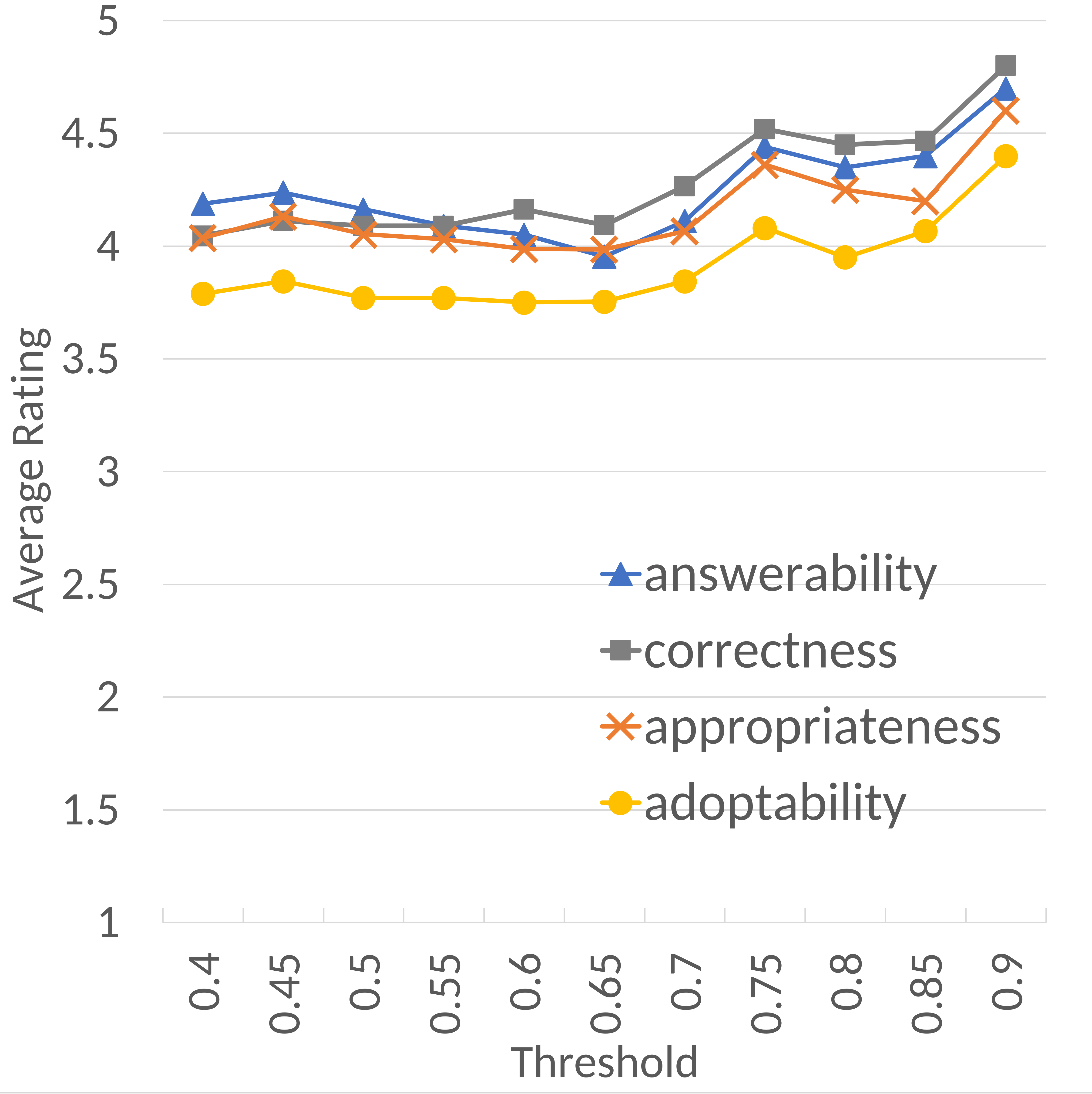
Participants were asked to rate the prospective pedagogical value of proposed questions using four evaluation metrics on a 5-point Likert scale that we developed for the current study: answerability, correctness, appropriateness, and adoptability.

Answerability refers to whether the question can be answered from the information shown in the proposed paragraph. Correctness is whether the proposed answer adequately addresses the question. Appropriateness is whether the question is appropriate for helping students achieve the corresponding learning objective. Adoptability is how likely the participants would adapt the proposed question to their class.

Each individual participant rated all 100 survey items. The questions used in the survey were created either by Quadl, Info-HCVAE, or a human expert. There were 34 questions generated by QUADL, 33 questions by Info-HCVAE, and 33 human-generated questions from the same OLI A&P course. Since the survey did not mention the source of the included questions, the participants blindly evaluated the prospective pedagogical value of those questions.

Consequently, five responses per question were collected, which is notably richer than any other human-rated study for question generation in the current literature, as these studies often involve only two coders.

Results: Question generation

Our primary research questions regarding the use of VELR with Quadl are: (1) How does VELR improve the accuracy (token precision) of the answer prediction? (2) How pedagogically adequate are the questions generated by QUADL when combined with VELR?

Accuracy of Answer Prediction Model. To investigate how VELR improved the accuracy of the answer prediction model used in Quadl, we evaluated the token precision with different threshold values.

We operationalized the accuracy of target token identification using two metrics: token precision and token recall. Token precision is the number of correctly predicted tokens divided by the number of tokens in the prediction. Token recall is the number of correctly predicted tokens divided by the number of ground truth tokens. For example, suppose a sentence “The target tissues of the nervous system are muscles and glands” has the ground truth tokens as “muscles and glands.” When the predicted token is “glands,” the token precision is 1.0 and recall is 0.33.

Figure 3 shows the change of token precision (a) and token recall (b) depending on the threshold when VELR is applied on 10 answer prediction models vs. 400 models. The figure shows the aggregated average over 7 runs.

Figure 3-a shows that VELR improves the token precision of the answer prediction model. When VELR is not used, the average token precision was 0.38 (as shown in the black dashed line). When VELR was used with a threshold of 0.6, for example, the token precision was 0.63.

There was a trade-off between precision and recall as predicted. As Figure 3-b shows the token recall decreased when the threshold increased$.$ The plots in the figure also suggest that there was no significant difference between 10 models and 400 models when unified voting was applied.

In sum, VELR improved the performance of the answer prediction model (which is based on the BERT architecture) even when it was trained with only 350 data points. For uniform voting, the number of models did not significantly impact the performance of the ensemble model. Due to the rejection, there is a clear trade-off between the soundness (token precision) and the completeness (token recall) of the ensemble model prediction.

As discussed before, the use of VELR is beneficial for tasks where soundness is valued over completeness—for pedagogical question generation, it is far more useful to generate a small number of pedagogically valuable questions than to generate lots of harmful questions. So, a further research question is: How pedagogically adequate are the questions generated by Quadl when combined with VELR?

Quality of the generated questions. The results on the answer prediction model shown above promisingly suggest that VELR has a practical application for generating questions for existing online courseware. The current survey results supported this expectation. Table 1 shows the survey results.

To see if there was a difference in ratings between questions with the different sources (Quadl vs. Infor-HCVAE vs. Human), a one-way ANOVA was applied separately to each metric. The results revealed that source is a main effect for ratings on all four metrics; F(2, 97) = 36.38, 24.15, 26.11, and 25.03, for answerability, correctness, appropriateness, and adoptability, respectively. A post hoc analysis using Tukey’s test showed that there was a statistically significant difference between Quadl and Info-HCVAE; t(97)=1.87, 1.50, 1.52, 1.39 for each metric, p < 0.05 for all metrics. There was, however, no significant difference between Quadl and human-generated questions for each of the four metrics: t(97)=0.40, 0.25, 0.16, 0.25, p = 0.19, 0.53, 0.78, 0.45 respectively.

In sum, the results from the current survey data suggest that Quadl-generated questions were evaluated as on-par with human-generated questions when VELR is applied to the answer prediction model trained with an extremely small data regime.

We further investigated how the consensus certainty of ensemble prediction of the answer prediction model impacted the quality of the generated questions. We sampled a subset of questions used in the survey by excluding the questions whose source target sentences would have been rejected if a threshold higher than $0.4$ had been applied. In other words, we investigated the following research question: How does the rejection threshold used by VELR when applied to the answer prediction model impact the ratings of the Quadl-generated questions? We plotted how the ratings change if thresholds higher than 0.4 were applied (Figure 6 in Appendix). The figure shows a trend that the participants would have increased their rating when higher values for rejection threshold were used, though the differences were relatively small and not monotonic.

Discussion and Limitations

Building a valid prediction model with extremely low data regimes is an omnipresent challenge in education research and many other domains when human annotation is required. Therefore, developing a data-agnostic technique to overcome this issue is vital to advance the pragmatic theory of learning engineering.

We proposed a voting function based on the distribution of the predicted posterior probability (or “certainly”). The experiment with CIFAR-10 showed that both min-majority and uniform voting can achieve better accuracy than the state-of-the-art method, DADA [36], even without any regulation or data augmentation technique on the image classification task.

Although concepts of soft-voting and classification with rejection have already been studied in the current literature, VELR is the first in the literature that combines soft-voting technique with rejection to carry out ensemble learning to overcome the issue of overfitting when a model is trained with an extremely low data regime.

In this paper, we explored only the Gaussian mixture model for min-majority voting, there are various ways to implement a voting technique by fitting different probability distributions. We conjecture that using a voting technique that better estimates a distribution of the posterior probability will further expand the potential of the proposed ensemble method.

We demonstrated that VELR is useful for a real-world application: pedagogical question generation as a learning-engineering tool for online courseware creation. However, the observations related to the evaluation of VELR on Quadl needs some attention. Since the total number of Quadl-generated questions used in the survey is small (34) due to the cost of the human-evaluation, the number of questions included in a subset when a higher threshold was applied was significantly small, too (Figure 6 in Appendix). The survey study should be replicated with a larger number of questions to further validate the current findings.

Conculsion

We found that combining soft voting among overfitting models and rejection based on the distribution of the learned posterior probability leads to remarkable accuracy on tasks even when models were trained with extremely low data regimes and were hence severely overfit.

While a conventional solution for overfitting due to extremely low data regimes is to restrict the flexibility of the model or increase the amount of data using the data-augmentation techniques, proposed VELR (Voting-based Ensemble Learning with Rejection) applies to any task and any models that estimate predicted certainly using posterior probability. VELR combines multiple overfitting models to output reliable predictions rather than preventing a model from overfitting while training.

The extremely low data regime is one of the most common problems in many practical tasks including educational data mining. Yet, building a reliable machine-learning model with a limited amount of data is an unavoidable demand. Further research to study the theoretical foundation for overcoming the overfitting problem under an extremely low data regime is therefore needed.

ACKNOWLEDGEMENTS

The research reported here was supported by National Science Foundation Grant No. 2016966 and No.1623702 to North Carolina State University.

REFERENCES

1. Abdi, H., & Williams, L. J. (2010). Principal component analysis. Wiley interdisciplinary reviews: computational statistics, 2(4), 433-459.
2. Amin-Naji, M., Aghagolzadeh, A., & Ezoji, M. (2020). CNNs hard voting for multi-focus image fusion. Journal ofAmbient Intelligence and Humanized Computing, 11(4), 1749-1769.
3. Anaby-Tavor, A., Carmeli, B., Goldbraich, E., Kantor, A., Kour, G., Shlomov, S., . . . Zwerdling, N. (2020). Do not have enough data? Deep learning to the rescue! Paper presented at the Proceedings of the AAAI Conference on Artificial Intelligence.
4. Chrysos, G. G., Kossaifi, J., & Zafeiriou, S. (2020). Rocgan: Robust conditional gan. International Journal of Computer Vision, 128(10), 2665-2683.
5. Cubuk, E. D., Zoph, B., Mane, D., Vasudevan, V., & Le, Q. V. (2019). Autoaugment: Learning augmentation strategies from data. Paper presented at the Proceedings of the IEEE/CVF Conference on Computer Vision and Pattern Recognition.
6. Dai, Z., Yang, Z., Yang, F., Cohen, W. W., & Salakhutdinov, R. R. (2017). Good semi-supervised learning that requires a bad gan. Advances in neural information processing systems, 30.
7. Dempster, A. P., Laird, N. M., & Rubin, D. B. (1977). Maximum likelihood from incomplete data via the EM algorithm. Journal of the Royal Statistical Society: Series B (Methodological), 39(1), 1-22.
8. Devlin, J., Chang, M.-W., Lee, K., & Toutanova, K. (2018). Bert: Pre-training of deep bidirectional transformers for language understanding. arXiv preprint arXiv:1810.04805.
9. Domingos, P. (2000). Bayesian averaging of classifiers and the overfitting problem. Paper presented at the ICML.
10. Dong, J., & Lin, T. (2019). Margingan: Adversarial training in semi-supervised learning. Advances in neural information processing systems, 32.
11. Ghosh, R., & Motani, M. (2021). Network-to-Network Regularization: Enforcing Occam's Razor to Improve Generalization. Advances in neural information processing systems, 34.
12. Kingma, D. P., Mohamed, S., Jimenez Rezende, D., & Welling, M. (2014). Semi-supervised learning with deep generative models. Advances in neural information processing systems, 27.
13. Krizhevsky, A., & Hinton, G. (2009). Learning multiple layers of features from tiny images.
14. Krizhevsky, A., Sutskever, I., & Hinton, G. E. (2012). Imagenet classification with deep convolutional neural networks. Advances in neural information processing systems, 25.
15. Li, C., Xu, T., Zhu, J., & Zhang, B. (2017). Triple generative adversarial nets. Advances in neural information processing systems, 30.
16. Liu, B., Wei, Y., Zhang, Y., & Yang, Q. (2017). Deep Neural Networks for High Dimension, Low Sample Size Data. Paper presented at the IJCAI.
17. Matsuda, N., Shimmei, M., Chaudhuri, P., Makam, D., Shrivastava, R., Wood, J., & Taneja, P. (in press). PASTEL: Evidence-based learning engineering methods to facilitate creation of adaptive online courseware. In F. Ouyang, P. Jiao, B. M. McLaren, & A. H. Alavi (Eds.), Artificial Intelligence in STEM Education: The Paradigmatic Shifts in Research, Education, and Technology (pp. 1-16). New York, NY: CSC Press.
18. Mikołajczyk, A., & Grochowski, M. (2018). Data augmentation for improving deep learning in image classification problem. Paper presented at the 2018 international interdisciplinary PhD workshop (IIPhDW).
19. Miyato, T., & Koyama, M. (2018). cGANs with projection discriminator. arXiv preprint arXiv:1802.05637.
20. Neelakantan, A., Vilnis, L., Le, Q. V., Sutskever, I., Kaiser, L., Kurach, K., & Martens, J. (2015). Adding gradient noise improves learning for very deep networks. arXiv preprint arXiv:1511.06807.
21. Ni, C., Charoenphakdee, N., Honda, J., & Sugiyama, M. (2019). On the calibration of multiclass classification with rejection. Advances in neural information processing systems, 32.
22. Noh, H., You, T., Mun, J., & Han, B. (2017). Regularizing deep neural networks by noise: Its interpretation and optimization. Advances in neural information processing systems, 30.
23. Qi, W., Yan, Y., Gong, Y., Liu, D., Duan, N., Chen, J., . . . Zhou, M. (2020, November). ProphetNet: Predicting Future N-gram for Sequence-to-SequencePre-training. Paper presented at the Findings of the Association for Computational Linguistics: EMNLP 2020, Online.
24. Rajpurkar, P., Zhang, J., Lopyrev, K., & Liang, P. (2016). Squad: 100,000+ questions for machine comprehension of text. arXiv preprint arXiv:1606.05250.
25. Salman, S., & Liu, X. (2019). Overfitting mechanism and avoidance in deep neural networks. arXiv preprint arXiv:1901.06566.
26. Sanyal, A., Dokania, P. K., Kanade, V., & Torr, P. H. (2020). How benign is benign overfitting? arXiv preprint arXiv:2007.04028.
27. Shimmei, M., Bier, N., & Matsuda, N. (to appear). Machine-Generated Questions Attract Instructors when Acquainted with Learning Objectives Paper presented at the Proceedings of the International Conference on Artificial Intelligence in Education.
28. Song, K., Tan, X., Qin, T., Lu, J., & Liu, T.-Y. (2020). Mpnet: Masked and permuted pre-training for language understanding. Advances in neural information processing systems, 33, 16857-16867.
29. Srivastava, N., Hinton, G., Krizhevsky, A., Sutskever, I., & Salakhutdinov, R. (2014). Dropout: a simple way to prevent neural networks from overfitting. The Journal of Machine Learning Research, 15(1), 1929-1958.
30. Van Engelen, J. E., & Hoos, H. H. (2020). A survey on semi-supervised learning. Machine Learning, 109(2), 373-440.
31. Wan, L., Zeiler, M., Zhang, S., Le Cun, Y., & Fergus, R. (2013). Regularization of neural networks using dropconnect. Paper presented at the International conference on machine learning.
32. Yang, T., Zhu, S., & Chen, C. (2020). Gradaug: A new regularization method for deep neural networks. Advances in neural information processing systems, 33, 14207-14218.
33. Yang, X., Song, Z., King, I., & Xu, Z. (2021). A survey on deep semi-supervised learning. arXiv preprint arXiv:2103.00550.
34. Yang, Y., Malaviya, C., Fernandez, J., Swayamdipta, S., Bras, R. L., Wang, J.-P., . . . Downey, D. (2020). Generative data augmentation for commonsense reasoning. arXiv preprint arXiv:2004.11546.
35. Yang, Z., Dai, Z., Yang, Y., Carbonell, J., Salakhutdinov, R. R., & Le, Q. V. (2019). Xlnet: Generalized autoregressive pretraining for language understanding. Advances in neural information processing systems, 32.
36. Zhang, X., Wang, Z., Liu, D., & Ling, Q. (2019). Dada: Deep adversarial data augmentation for extremely low data regime classification. Paper presented at the ICASSP 2019-2019 IEEE International Conference on Acoustics, Speech and Signal Processing (ICASSP).
37. Zhou, Z.-H. (2012). Ensemble methods: foundations and algorithms: CRC press.

Appendix

Classification model for CIFAR-10

Each model was trained for 9000 steps. The batch size was 32. The learning rate was 10^-3. No regularization technique was used.

Trade-off between Accuracy and Predicted Ratio

The dotted line and solid line show min-majority and uniform voting, respectively. Each voting schema has three plots with 100, 1000, and 5000 models as shown with different markers. Each line contains 20 data points (denoted as markers on the line). Each data point corresponds to a particular threshold ranging from 0.95 to 0.0 (i.e., no rejection), decreasing by 0.5. Since the predicted ratio increases as the threshold is lowered, the 20 data points on the line are coincidentally arranged in a decremental manner, from left to right, for the threshold (hence the threshold values are not displayed on the plot for simplicity). For example, the second marker from the right on min-majority models shows that when θ = 0.90, the min-majority voting over 1000 models yielded the accuracy of 0.49 with the predicted ratio of 0.62.

The figure shows uniform voting was clearly better than a single model prediction, and consistently better than or equal to min-majority voting.

(a) 200 samples per class

(b) 1000 samples per class

Overview of QUADL

The answer prediction model identifies start/end index <Is, Ie> of the target token (i.e., key term) in S. When S is not suitable for LO, it outputs <0,0>. The question conversion model converts S with target token to a verbatim question.

Change of Average Rating for Questions Generated by QUADL

Figure 6 was plotted to answer the research question: How does the rejection threshold used by VELR when applied to the answer prediction model impact the ratings of the Quadl-generated questions?

Each data point includes a subset of questions used in the survey excluding the questions whose source target sentences would have been rejected if a threshold higher than $0.4$ had been applied.

The figure shows how the ratings change if thresholds higher than 0.4 were applied. The figure shows a trend that the participants would have increased their rating when higher values for rejection threshold were used, though the differences were relatively small and not monotonic. Appropriateness, for example, increased from 4.04 to 4.30 when the threshold was changed from 0.4 to 0.75. Accordingly, acceptability also increased from 3.53 to 4.10.

1. The code and data are available at https://github.com/IEClab-NCSU/VELR ↑

2. We use the term “posterior probability”, “prediction”, and “certainty” interchangeably unless otherwise noted. ↑

© 2023 Copyright is held by the author(s). This work is distributed under the Creative Commons Attribution-NonCommercial-NoDerivatives 4.0 International (CC BY-NC-ND 4.0) license.