ABSTRACT
This paper studies the problem of automatically adjusting the difficulty level of educational exercises to facilitate learning. Previous work on this topic either relies on large datasets or requires multiple interactions before it adjusts properly. Although this is sufficient for large-scale online courses, there are also scenarios where students are expected to only work through a few trials. In these cases, the adjustment needs to respond to only a few data points. To accommodate this, we propose a novel difficulty adjustment method that requires less data and adapts faster. Our proposed method refits an existing item response theory model to work on smaller datasets by generalizing based on attributes of the exercises. To adapt faster, we additionally introduce a discount value that weakens the influence of past interactions. We evaluate our proposed method on simulations and a user study using an example graph theory lecture. Our results show that our approach indeed succeeds in adjusting to learners quickly.
Keywords
1. INTRODUCTION
In computer-based learning, it is important to solidify newly learned content through exercises [16]. Appropriately tailoring the difficulty level of these exercises has a positive effect on learning gains and motivation [8, 23]. Exercises too difficult could lead to anxiety, whereas exercises too easy could lead to boredom, thus the importance of balance, dubbed the state of flow [10]. Consequently, there have been attempts to automatically adjust the difficulty in computer-based learning settings. Individual works refer to this idea using different keywords, such as computer adaptive practice [21, 29], adaptive curriculum [4], or personalized difficulty [41]. In this paper, we use the term Dynamic Difficulty Adjustment (DDA) [18, 26].
Many works on DDA for educational purposes focus on large-scale applications, similar to Massive Open Online Courses (MOOCs). In particular, most of them rely on one of two prerequisites. Either they require large prerecorded datasets to pre-train their models, which can mean up to months’ worth of data [4, 21], or they require many interactions per user until they start adapting well [21, 24, 28]. This is not suitable for cases where students only complete a limited number of exercises, for example, when introducing a new concept in higher math or logic. Educational DDA approaches that do not rely on large datasets or many iterations, often break down the learning objective into distinct Knowledge Components (KCs) that students should master [5, 9, 27]. However, defining these KCs can be a laborious task that requires extensive expertise in the subject matter [22]. In certain cases, it is more straightforward to identify exercise attributes instead. For example, in arithmetic exercises, key attributes might include the magnitude of numbers involved or the number of computational steps required. In graph theory, difficulty may hinge on the graph’s size and complexity.
For cases where exercise attributes are easier to define than KCs, we propose a novel DDA algorithm based on Item Response Theory (IRT) that alleviates the aforementioned problems of few iterations and small datasets. IRT models are used to predict students’ future success in a task based on past interactions [20]. In DDA they can be used to provide a user with exercises that they can solve with a predefined success probability. Traditional IRT models assume that the students have a constant ability level. To fix this, we introduce a discount factor that weakens the influence of past interactions. Because of the lack of massive datasets, the model cannot learn the difficulty of each exercise individually as IRT-based approaches normally do. By adapting the IRT model to be trained on exercise attributes, our algorithm can generalize the difficulty between exercises. We test our proposed method on an example graph theory lecture with both simulations and a user study. In both experiments, our algorithm succeeds in quickly adjusting the difficulty so that the students obtain our defined success rate.
2. RELATED WORKS
Current DDA methods for exercises in educational settings can be divided into four major techniques. The first category is adapting the difficulty based on handcrafted scoring systems [3, 33, 34]. Here, the students get a score for each completed exercise. This score is then compared to expert-written thresholds to decide which difficulty level will be provided to the student next. The downside of such approaches is that a lot of domain knowledge and time is needed to handcraft good scoring systems for different topics.
The second category is based on the field of Knowledge Tracing (KT). KT addresses the problem of predicting the student’s success on an unseen future task given the history of his learning and task attempts [1]. For DDA, KT can be used to predict the success rate of each possible exercise and provide the most suitable one to the student. Leyzberg et al. [24] and Schodde et al. [36], for example, do so by using Bayesian Knowledge Tracing (BKT) which models how likely it is that a student already learned different KCs. Aside from BKT, other models that require KCs to represent exercises include Performance Factor Analysis (PFA) [27] and Additive Factor Model (AFM) [5, 6]. Based on this, BKT, PFA, and AFM can provide exercises for KCs that the student likely has not learned yet. However, if exercises are not distinguishable by different KCs, these models cannot select suitable exercises because all the exercises would be equivalent to the model. In such scenarios, a KT model that can distinguish exercises without relying on KCs is required. The most prominent examples of this are Item Response Theory models (IRT) like the One-Parameter Logistic (1PL) [31] or Four-Parameter Logistic (4PL) [2] model. These models work by learning an ability value for the student and comparing it to the learned difficulty values of each exercise. However, these models are not suitable for DDA since they assume that the student’s ability is constant.
The third category of DDA approaches in educational settings is based on the ELO system. ELO was first introduced for chess [14] where it assigns a rating for each player and tries to pit players with similar ratings against each other. After each interaction, the ratings are updated. Klinkenberg et al. [21] were the first to use ELO for DDA. Instead of modeling the ratings of different players, they assign a rating to each individual exercise and each student using the ELO system. In this way, students can be given exercises that match their rating. Recent years saw several variations of ELO-based DDA for education [28, 35, 40]. However, for the scenario we envision, there are two main drawbacks. First, these ELO-based systems require datasets with several repetitions of each individual exercise to learn their individual difficulty rating, with [28] requiring 100 interactions per exercise item. Second, the learning rate in the ELO system is scenario-dependent. Handcrafting such a value is difficult when the goal is fast adaptation without overshooting.
The final category of DDA approaches for education use Reinforcement Learning (RL). Belfer et al. [4] and Zhang et al. [41] use RL to directly choose individual actions that should be provided to the student next. However, both of their approaches require extensive datasets to pre-train their models. Clement et al. [7] used RL to decide whether there should be another more difficult exercise for the same KC or an exercise for another KC. This requires experts to design a carefully crafted curriculum with multiple paths that covers all possible scenarios, which is not feasible for many applications. Another drawback of RL-based DDA approaches is that they require long sequences of interactions to be able to explore different state-action pairs before they can adapt to the student. This makes them unsuitable for scenarios with a limited number of interactions.
In addition to education, there is also a large amount of work on DDA in games. Because of the quick pace of games, many DDA techniques in games can afford to use large amounts of interactions and data [39].For example, Moon et al. [25] used 60.2M data points for pre-training. However, there also have been works on DDA for games that focus on fast adaptation using little data. One group of work here used procedural content generation [11, 12, 17]. These methods rely, at least in part, on the ability to procedurally generate game levels based on the previous game level. This is not possible for many educational scenarios where exercises are handcrafted by experts. Finally, Fernandes and Levieux [15] aim to quickly adapt to players without using any prerecorded data points. To this end, they use the first 20 interactions of each new player to generate a dataset for logistic regression. While this is feasible for fast-paced games, it requires too many interactions to work with topics like math or logic, where each exercise may take minutes.
We propose a new DDA approach to address the drawbacks of the aforementioned approaches for cases where it is hard to define KCs and only a limited number of exercises and prerecorded data is available. We use an IRT model based on attributes to learn the difficulty values for all exercises based on a limited set of prerecorded data points. To quickly adapt to new students, we add a discount value to the model update to weaken IRT’s assumption of constant skill.
3. APPROACH
To adjust the difficulty, we need a model that describes the student’s behavior, and then a method to decide on the difficulty based on that. We describe this process in the following.
3.1 Student Model
The student model contains a set of student attributes and provides the probability of observing each possible student action. In our case, the set of possible actions is the success of or failure to solve an exercise. For our educational scenario, we find that the 4PL model [2] is a good fit. It is feasible to train on small-scale datasets. It also models the guess and slip probabilities - the chances of accidentally getting the exercise right or wrong - which is an inherent feature of the kind of exercises we work with. The original 4PL model, describing the probability of a student \(u_i\) solving an exercise \(q_j\), is written in Equation 1. \begin {equation} p_{solve}(u_i, q_j) = c + (d - c)\frac {1}{1 + e ^ {-a_j(\theta _i - b_j)}} \label {eq:4pl} \end {equation} where \(\theta _i\) describes the student’s ability, \(a_j\) defines the discriminatory power of the exercise, i.e. how sharply the exercise can distinguish students of different ability levels, \(b_j\) the exercise difficulty, \(c\) the probability that the user guesses the correct answer, and \(d\) the probability that the user does not slip with a wrong answer. In our scenario where all the exercises are of the same nature, we find that every exercise should have the same discriminatory power. Therefore, we learn a single value of \(a\) that applies to every exercise \(j\). The difficulty \(b_j\) will also not be learned separately for each exercise, as each exercise in our dataset has far too few samples. Instead, we calculate \(b_j\) from the attributes of our exercises which will be explained in Section 4.1. This is done by learning weights \(\vec {w}\) for the attributes: \begin {equation} b_j = \vec {{attr}_j} \cdot \vec {w} \end {equation} where \(\vec {{attr}_j}\) is the vector listing the attributes of the exercise, for example, the number of vertices and edges of a graph. Through this, we learn a shared set of weights for all the exercises instead of learning \(b_j\) for each exercise individually.
3.2 Training Exercise Parameters
We separate the training process of our model into two steps. The first step is fitting the global parameters of the exercises on prerecorded data. The second step is to fit the student ability of each student during deployment. This two-step training is inspired by Xu et al. [38] and has been shown to work well and efficiently. The model we train in the first step is the original 4PL model. The parameters we want from this are the attribute weights \(\vec {w}\) and the \(a, c, d\) values from the 4PL model introduced in Section 3.1. Naturally, we do need to include the student ability \(\theta \) for the training to work, but we will not use this \(\theta \) further after training. We optimize the joint maximum likelihood of all student’s past actions using gradient descent, similar to Warm et al. [37]: \begin {equation} L = \sum _{(u_i, q_j, y_{solve}, t) \in \mathscr {D}}l(y_{solve}, p_{solve}(u_i, q_j)), \label {eq:4pl-loss} \end {equation} where the tuple \((u_i, q_j, y_{solve}, t)\) represents the event of student \(u_i\) making an attempt on exercise \(q_j\) with success outcome \(y_{solve} \in \{0, 1\}\) at time step \(t \in \mathbb {N}\) and \(l(\cdot , \cdot )\) is the cross-entropy loss. This describes the first step of training, which uses prerecorded data.
3.3 User Ability Update & Difficulty Adjustment
When deploying the DDA model to a new student, we fix the exercise parameters \(\vec {w}, a,c,\) and \(d\) learned in Section 3.2. We only learn the student’s ability value \(\theta \). Every time the student finishes an exercise, we run gradient descent on all observed attempts by this student until it converges or reaches a maximum number of 1,000 iterations.
One caveat of the original 4PL model is that it assumes that students have an unchanging ability level. This does not reflect how students learn a new concept. To remedy this, we add a discount value \(\gamma \in (0, 1)\) to our maximum likelihood function (Equation 3). With this, we weigh the past actions by \(\gamma ^{T-t}\), where \(T\) is the current time step and \(t\) is that action’s time step. By giving less weight to past evidence, we make the change in ability level more fluid and more reliant on recent outcomes. The loss function we optimize for becomes \begin {equation} L = \sum _{(u_i, q_j, y_{solve}, t) \in \mathscr {D}, t < T}{\gamma ^{T - t} l(y_{solve}, p_{solve}(u_i, q_j))}. \label {eq:discount-loss} \end {equation} After the ability value is updated, the probability of solving \(p_{solve}\) is calculated for each exercise. The exercise with \(p_{solve}\) closest to a desired success rate is chosen and provided to the student next. For this, we need to pick the success rate that the students should get. Gonzalez-Duque et al. [11] suggest a success rate between 50% and 70%, while Klinkenberg et al. [21] suggest 75%. Therefore we tested our DDA approach using smaller pilot studies with a target success rate of 70%, 65%, and 60%. Since both 70% and 65% provided too easy exercises, we opted for 60% for our final study.
4. EXPERIMENTS
4.1 Task
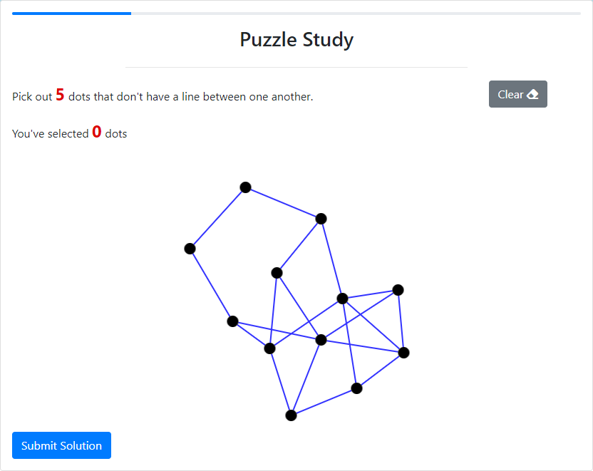
For our experiments, we use an example graph theory lecture, where students are introduced to the Maximum Independent Set (MIS) of a graph (i.e., the largest set of vertices such that none of the selected vertices are adjacent to one another). It is a concept in graph theory that students need to be familiar with, therefore the setting simulates a real learning scenario. Furthermore, most people have not heard of MIS before, so it is a newly introduced concept. Finally, the definition of the MIS is simple, yet finding an MIS for a given graph is difficult. It requires an intuition that is best built through exercises. To this end, we generate a pool of 191 exercises that can be provided to the students. Figure 1 shows an example of such an exercise during our study.
4.2 Training the DDA Model
We trained our model as described in Section 3. To learn the difficulty \(b_j\) of each exercise we use the attributes \(\vec {{attr}}= (|V_{MIS}|, p_{alg}, |V|,|E|,|I|)\), where \(|V|\) and \(|E|\) are the number of vertices and edges in the graph, \(|V_{MIS}|\) is the size of the MIS, \(p_{alg}\) is the success rate of a stochastic solver algorithm on this graph (see Appendix A), and \(|I|\) is the number of intersections of edges. To pre-train our DDA model, we collected data from 80 users without using DDA. For details of the training parameters and the data collection see Appendix B.
4.3 Simulation Design
Before starting the user study, we carry out experiments with simulations to verify that our algorithm works in adjusting to simulated students’ behavior. We handcrafted simulated students that interact with the DDA algorithm. Our simulated students have an internal ability value. If the ability value plus a Gaussian noise is greater than the exercise’s difficulty, then the attempt is a success. Otherwise, it is a failure. The ability value is increased by learning, which happens when the exercise is given at the right level of difficulty in accordance with Vygotsky’s zone of proximal development [32]. The student also has a boredom and anxiety value, which increase when an exercise is too easy or too hard, respectively. Learning only occurs when the sum of boredom and anxiety values is lower than a set threshold. For details refer to the repository that contains our implementation and data 1. To emulate our user study (see Section 4.4), the simulation starts with three fixed pre-test exercises, where the DDA algorithm updates its student model but does not choose the exercises. Then it loops through 12 training exercises that are chosen by the DDA algorithm.
4.4 User Study Design
Procedure: In our user study, the participants are presented with a sequence of MIS exercises, divided into three phases: pre-test, training, and post-test. Before the experiment, there is a questionnaire for the participant’s demographics and their general interest in puzzles, computer science, and mathematics. After that, the students are provided with a tutorial that resembles the part of a graph theory lecture that introduces Maximum Independent Sets (MIS). This also includes a tutorial exercise to make sure that the participants understood the task correctly. The pre- and post-test phases are fixed and each contains one exercise of easy, medium, and hard difficulty based on a handcrafted difficulty metric (see Appendix A). The tests provide bonus payments and are used to motivate participants to practice. The training phase consists of 12 exercises where our proposed algorithm (see Section 3) runs in the background to estimate the student’s ability and provides exercises that the student is estimated to have a 60% probability of solving. After the post-test, there is another free-text questionnaire asking about the task difficulty and the student’s feelings about the task. For each exercise, the participant sees the graph and the number of vertices that need to be selected (Figure 1). The exercise will not be declared solved automatically once the correct vertices are chosen, but the participant has to manually click “Submit”. They are told that there is a time limit on each exercise but do not know how long it is (90 seconds). This is done to reduce the sensation of time and enable flow. We display a red flag 5 seconds before the time runs out to remind them to submit the solution if they think they have one. After submitting, there is a pop-up saying if the solution was correct. The median time the experiment took was 23 minutes.
Participants & Compensation: We recruited 30 participants using the online platform Prolific. They were required to be fluent in English. For some participants, the training exercises were too difficult overall and they failed to solve more than one training exercise. Removing those participants from the analysis left us with 25 participants. The participants included 15 males and 10 females, with ages ranging from 20 to 47 years old and a mean of 29.2. Each participant was paid £3.9 for successful participation. Additionally, for each correctly solved pre- and post-test exercise, they were paid £0.1 - 0.2, depending on the time they needed. This totals up to a potential bonus of £1.2.
Research Questions & Hypotheses: The main research question for our study was whether our DDA approach adapts as intended. For this, we hypothesized that there is no significant difference between the desired success rate (60%) and the actual success rate of the participants during the training phase. As a secondary research question, we are interested in investigating if our adapted IRT model is still useful for knowledge tracing. That would be the case if there is a correlation between the ability level that the student model within our DDA approach assigns to each participant after training and their performance in the post-test. This work presents the first part of a bigger study that we preregistered online. 2 To keep the scope of this work focused on the adaptation, we will describe the results of the remaining study in future work after a thorough analysis.
5. RESULTS
5.1 Result of the Simulations
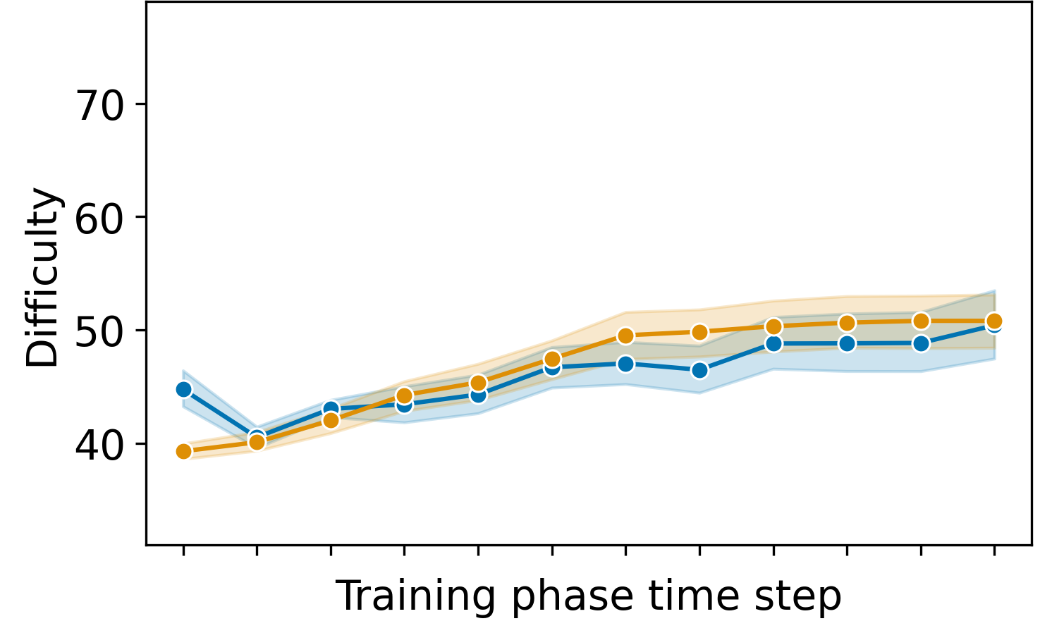
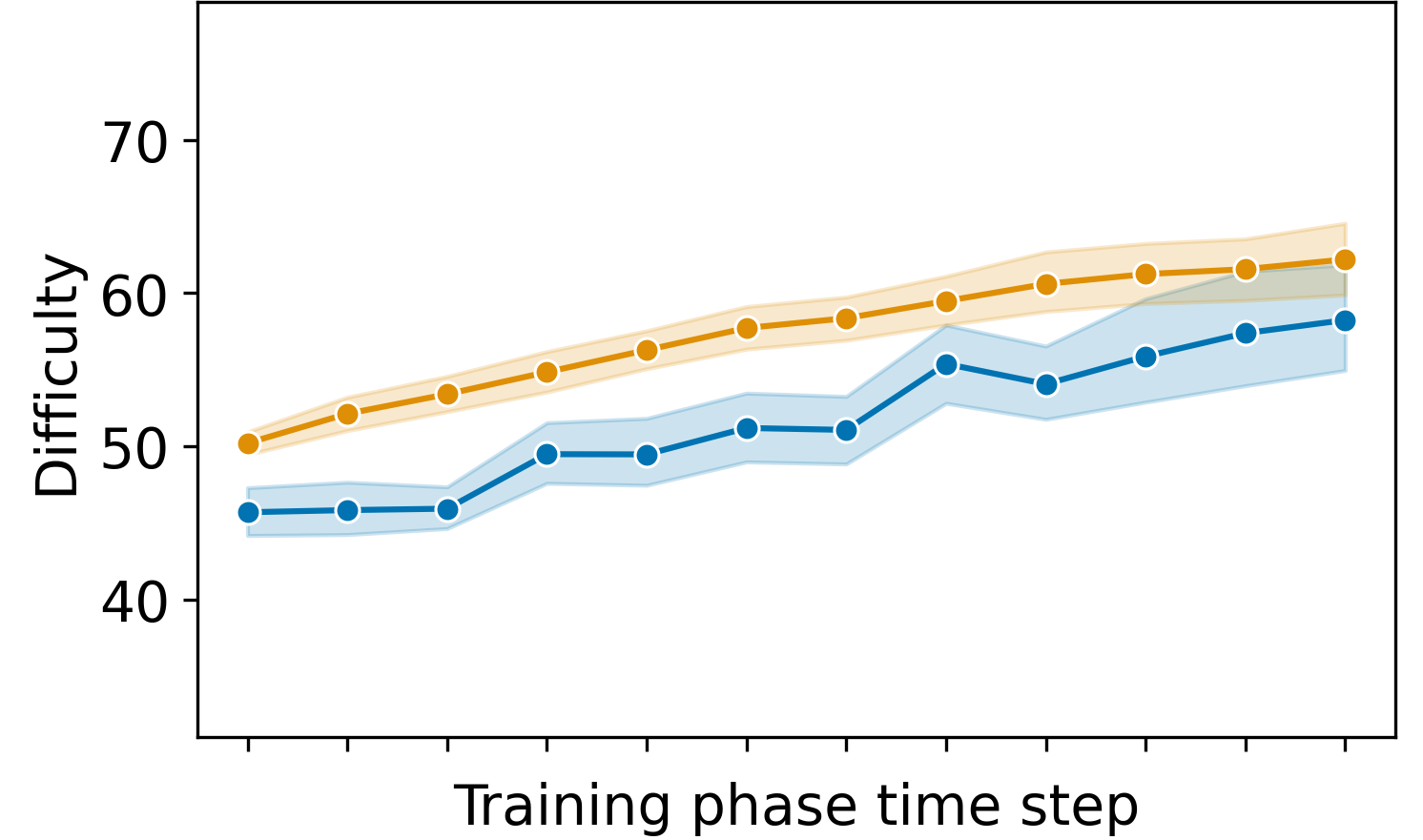
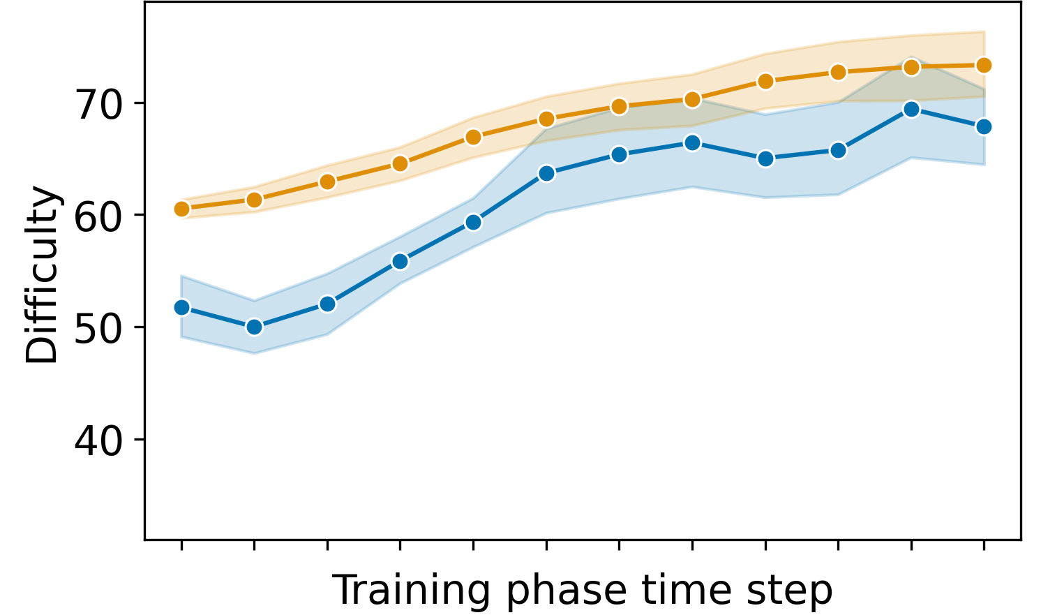
During the simulation, we used three groups of 50 simulated students where each group simulated students with a different initial ability level (low, medium, and high). To visualize how the DDA algorithm performs, we designed a handcrafted metric for the difficulty of each exercise (see Appendix A). Figure 2 shows the trajectory of the student’s ability and the difficulty of the exercises provided to them in each time step. Right up from the first time step of the training phase, there was a difference in the difficulties that the different students get because of the different pre-test results. The students with higher initial abilities got harder exercises. The difficulty was slightly lower than the student’s ability because we want to have a 60% success rate. As the users increased in their ability level with training, the difficulty of the exercises provided to the students also increased, showing the system can detect the change and adapt itself accordingly. Taking a look at the success rate of exercise solves during the training phase, the simulated students were able to solve 61.1% \(\pm \) 12.4% of the exercises. Using a one sample t-test, we find no significant difference from 60%; t(df) = 1.08, p = 0.28, Cohen’s d = 0.09. Also, DDA yielded higher learning than random and predefined difficulty curve baselines. Simulated students on DDA improved by a mean of 12.5 difficulty units between pre- and post-test, while predefined difficulty curve and random improve by 9.6 and 6.9 difficulty units, respectively.
5.2 Results of the User study
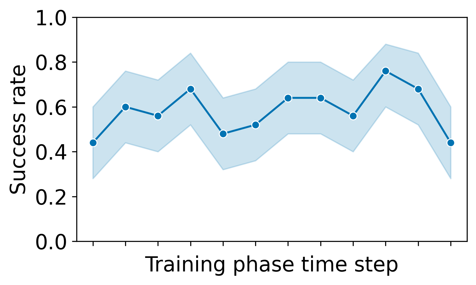
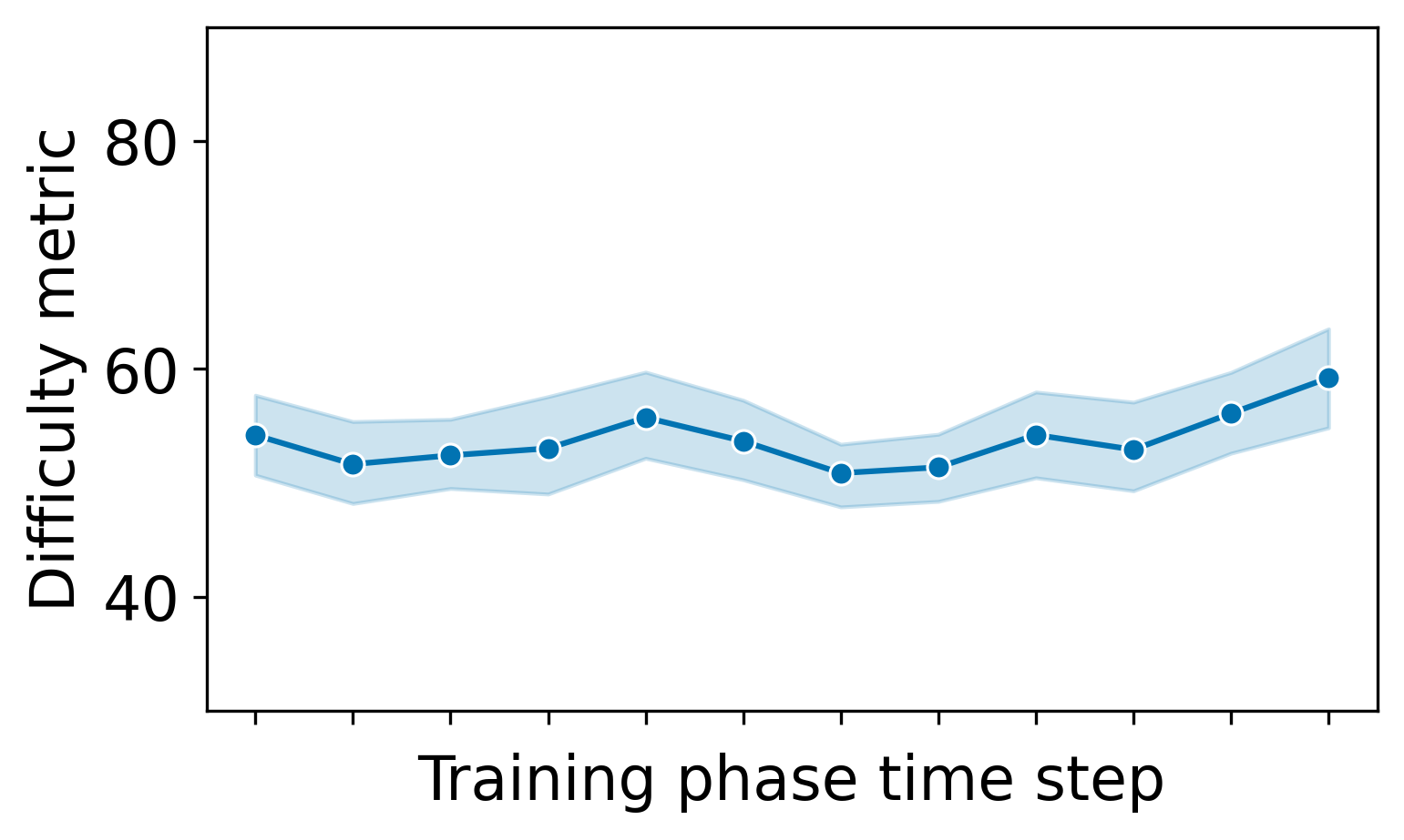
For our main research question, we wanted to verify that our approach was capable of providing exercises with a 60% success rate. Our participants successfully solved on average 7.0 \(\pm \) 1.2 out of 12 training exercises, which translates to a success rate of 58 \(\pm \) 10%. Using a one sample t-test, we find that the success rate was not significantly different from our aimed 60% with a very small effect size; t(df) = -0.86, p = 0.40, Cohen’s d = 0.17. For context, when collecting training data without DDA, the mean success rate was 49 \(\pm \) 20%. In Figure 3 we show the mean success rate and exercise difficulty during the training phase.
To see if our DDA approach can infer the student’s post-test performance from the training session, we calculated the Spearman correlation between the fitted ability value \(\theta \) after the training phase and the post-test score. We found significant correlations for the data collected without DDA ((\(r^2\) = 0.599, p = 0.003) for predefined difficulty and (\(r^2\) = 0.522, p = 0.006) for self-determined difficulty). For the data collected with DDA we found no significant correlation (\(r^2\) = 0.144, p = 0.49).
6. DISCUSSION
The main goal of this paper was to introduce a DDA algorithm that is able to quickly adapt to students after only a few interactions. During both our simulated and human user experiments we did not find a significant difference from the desired success rate of 60%, with very small effect sizes in both experiments. This indicates that there is no large difference between our outcome and the desired success rate. For simulated users, it also did so while staying in the zone of proximal development where our simulated users learned the most. This shows that it did not simply give very easy and very hard exercises to get the given quota but actually estimated the student’s chance of success for each exercise. For real users, the mean success rate hovered around 60% throughout the course of the experiment while the average difficulty increased towards the end (see Figure 3). This shows that the participants improved and that our DDA algorithm adapted to them correctly. As an example for individual students, we show and discuss the progression of two students in Appendix C. While previous user studies with many interactions managed to achieve their desired success rate [21], Schadenberg et al. [35] showed that this is not a trivial task for scenarios with limited numbers of interactions. In their user study, which used a similar amount of interactions as our study, they were not able to change the success rate compared to their baseline.
We also took a closer look at the \(5\) participants that we excluded from the initial evaluation because they did not get more than one exercise correct during training. Our DDA algorithm was correctly providing them with the easiest possible puzzle in each time step, but could not give them easier exercises because there just were no easier exercises in the pool. To alleviate this limitation, future applications could utilize this ability of the DDA algorithm to identify situations where students are struggling. Based on this automatic detection, a human teacher or tutor could intervene and provide further help individually.
We checked whether the participant’s \(\theta \) inferred during the training phase correlates with their post-test performance. We found that this correlation exists when the DDA does not choose the exercises, but not when we enforce a 60% success rate. This is in line with the findings by Eggen and Verschoor that the further the success rate is from 50%, the worse the IRT models estimate the performance [13].
Our work has some limitations. First, our approach is only suitable for problems that can be parameterized by attributes. Second, our modeling of student learning might be less nuanced than models based on KCs that can show how well the students know each KC. Finally, a direct comparison with algorithms like ELO or BKT as well as an investigation of the learning performance of the students is needed to fully grasp the contribution of our method. This was not within the scope of this work.
7. CONCLUSION & FUTURE WORK
In this work, we proposed a novel DDA algorithm for intelligent tutoring systems with a limited number of interactions and small datasets. We showed in simulations and a user study that our approach is able to achieve the desired success rate after limited interactions. In the future, we plan to evaluate how this influences the students’ learning process. Furthermore, future work should investigate the potential of DDA algorithms to detect situations where students require additional support.
8. ACKNOWLEDGMENTS
This research was partially supported by the Affective Computing & HCI Innovation Research Lab between Huawei Technologies and the University of Augsburg.
References
- G. Abdelrahman, Q. Wang, and B. P. Nunes. Knowledge tracing: A survey. ACM Comput. Surv., 55(11):224:1–224:37, 2023.
- M. A. Barton and F. M. Lord. An upper asymptote for the three-parameter logistic item-response model. ETS Research Report Series, 1981(1):i–8, 1981.
- K. N. Bauer, R. C. Brusso, and K. A. Orvis. Using adaptive difficulty to optimize videogame-based training performance: The moderating role of personality. Military Psychology, 24(2):148–165, 2012.
- R. Belfer, E. Kochmar, and I. V. Serban. Raising student completion rates with adaptive curriculum and contextual bandits. In International Conference on Artificial Intelligence in Education, pages 724–730. Springer, 2022.
- H. Cen, K. Koedinger, and B. Junker. Learning factors analysis–a general method for cognitive model evaluation and improvement. In Intelligent Tutoring Systems: 8th International Conference, ITS 2006, Jhongli, Taiwan, June 26-30, 2006. Proceedings 8, pages 164–175. Springer, 2006.
- H. Cen, K. Koedinger, and B. Junker. Comparing two irt models for conjunctive skills. In Intelligent Tutoring Systems: 9th International Conference, ITS 2008, Montreal, Canada, June 23-27, 2008 Proceedings 9, pages 796–798. Springer, 2008.
- B. Clement, D. Roy, P. Oudeyer, and M. Lopes. Multi-armed bandits for intelligent tutoring systems. In Proceedings of the 8th International Conference on Educational Data Mining, EDM 2015, Madrid, Spain, June 26-29, 2015, page 21. International Educational Data Mining Society (IEDMS), 2015.
- G. Corbalan, L. Kester, and J. J. Van Merriënboer. Selecting learning tasks: Effects of adaptation and shared control on learning efficiency and task involvement. Contemporary Educational Psychology, 33(4):733–756, 2008.
- A. T. Corbett and J. R. Anderson. Knowledge tracing: Modeling the acquisition of procedural knowledge. User modeling and user-adapted interaction, 4(4):253–278, 1994.
- M. Csikszentmihalyi. Flow: The psychology of optimal experience, volume 1990. Harper & Row New York, 1990.
- M. G. Duque, R. B. Palm, D. Ha, and S. Risi. Finding game levels with the right difficulty in a few trials through intelligent trial-and-error. In IEEE Conference on Games, CoG, pages 503–510, 2020.
- M. G. Duque, R. B. Palm, and S. Risi. Fast game content adaptation through bayesian-based player modelling. In IEEE Conference on Games, CoG, pages 1–8. IEEE, 2021.
- T. J. Eggen and A. J. Verschoor. Optimal testing with easy or difficult items in computerized adaptive testing. Applied Psychological Measurement, 30(5):379–393, 2006.
- A. E. Elo. The Rating of Chessplayers, Past and Present. Arco Pub., New York, 1978.
- W. R. Fernandes and G. Levieux. \delta -logit : Dynamic difficulty adjustment using few data points. In Entertainment Computing and Serious Games - First IFIP TC 14 Joint International Conference, ICEC-JCSG 2019, Arequipa, Peru, November 11-15, 2019, Proceedings, volume 11863 of Lecture Notes in Computer Science, pages 158–171. Springer, 2019.
- J. Hattie. Visible learning for teachers: Maximizing impact on learning. Routledge, 2012.
- T. Huber, S. Mertes, S. Rangelova, S. Flutura, and E. André. Dynamic difficulty adjustment in virtual reality exergames through experience-driven procedural content generation. In IEEE Symposium Series on Computational Intelligence, SSCI 2021, Orlando, FL, USA, December 5-7, 2021, pages 1–8, 2021.
- R. Hunicke. The case for dynamic difficulty adjustment in games. In Proceedings of the International Conference on Advances in Computer Entertainment Technology, ACE, pages 429–433, 2005.
- B. E. John and D. E. Kieras. The goms family of user interface analysis techniques: Comparison and contrast. ACM Transactions on Computer-Human Interaction (TOCHI), 3(4):320–351, 1996.
- M. M. Khajah, Y. Huang, J. P. González-Brenes, M. C. Mozer, and P. Brusilovsky. Integrating knowledge tracing and item response theory: A tale of two frameworks. In CEUR Workshop proceedings, volume 1181, pages 7–15. University of Pittsburgh, 2014.
- S. Klinkenberg, M. Straatemeier, and H. L. van der Maas. Computer adaptive practice of maths ability using a new item response model for on the fly ability and difficulty estimation. Computers & Education, 57(2):1813–1824, 2011.
- V. Kodaganallur, R. R. Weitz, and D. Rosenthal. A comparison of model-tracing and constraint-based intelligent tutoring paradigms. Int. J. Artif. Intell. Educ., 15(2):117–144, 2005.
- D. Kostons, T. van Gog, and F. Paas. Self-assessment and task selection in learner-controlled instruction: Differences between effective and ineffective learners. Computers & Education, 54(4):932–940, 2010.
- D. Leyzberg, S. Spaulding, and B. Scassellati. Personalizing robot tutors to individuals’ learning differences. In 2014 9th ACM/IEEE International Conference on Human-Robot Interaction (HRI), pages 423–430. IEEE, 2014.
- H. Moon and J. Seo. Dynamic difficulty adjustment via fast user adaptation. In UIST ’20 Adjunct: The 33rd Annual ACM Symposium on User Interface Software and Technology, Virtual Event, USA, October 20-23, 2020, pages 13–15. ACM, 2020.
- O. Pastushenko. Gamification in assignments: Using dynamic difficulty adjustment and learning analytics to enhance education. In Extended Abstracts of the Annual Symposium on Computer-Human Interaction in Play Companion Extended Abstracts, CHI PLAY ’19 Extended Abstracts, page 47–53, New York, NY, USA, 2019. Association for Computing Machinery.
- P. I. Pavlik, H. Cen, and K. R. Koedinger. Performance factors analysis - A new alternative to knowledge tracing. In V. Dimitrova, R. Mizoguchi, B. du Boulay, and A. C. Graesser, editors, Artificial Intelligence in Education: Building Learning Systems that Care: From Knowledge Representation to Affective Modelling, Proceedings of the 14th International Conference on Artificial Intelligence in Education, AIED 2009, July 6-10, 2009, Brighton, UK, volume 200 of Frontiers in Artificial Intelligence and Applications, pages 531–538. IOS Press, 2009.
- R. Pelánek. Applications of the elo rating system in adaptive educational systems. Computers & Education, 98:169–179, 2016.
- R. Pelánek, J. Papoušek, J. Řihák, V. Stanislav, and J. Nižnan. Elo-based learner modeling for the adaptive practice of facts. User Modeling and User-Adapted Interaction, 27(1):89–118, 2017.
- E. Poromaa. Crushing candy crush : Predicting human success rate in a mobile game using monte-carlo tree search. 2017.
- M. D. Reckase. Unifactor latent trait models applied to multifactor tests: Results and implications. Journal of educational statistics, 4(3):207–230, 1979.
- M. M. Rohrkemper. Self-regulated learning and academic achievement: A vygotskian view. In Self-regulated learning and academic achievement, pages 143–167. Springer, 1989.
- C. Romero, S. Ventura, E. L. Gibaja, C. Hervás, and F. Romero. Web-based adaptive training simulator system for cardiac life support. Artificial Intelligence in Medicine, 38(1):67–78, 2006.
- R. J. Salden, F. Paas, and J. J. Van Merriënboer. Personalised adaptive task selection in air traffic control: Effects on training efficiency and transfer. Learning and Instruction, 16(4):350–362, 2006.
- B. R. Schadenberg, M. A. Neerincx, F. Cnossen, and R. Looije. Personalising game difficulty to keep children motivated to play with a social robot: A bayesian approach. Cognitive systems research, 43:222–231, 2017.
- T. Schodde, K. Bergmann, and S. Kopp. Adaptive robot language tutoring based on bayesian knowledge tracing and predictive decision-making. In Proceedings of the 2017 ACM/IEEE International Conference on Human-Robot Interaction, pages 128–136, 2017.
- T. A. Warm. Weighted likelihood estimation of ability in item response theory. Psychometrika, 54(3):427–450, 1989.
- L. Xu and M. A. Davenport. Dynamic knowledge embedding and tracing. In A. N. Rafferty, J. Whitehill, C. Romero, and V. Cavalli-Sforza, editors, Proceedings of the 13th International Conference on Educational Data Mining, EDM 2020, Fully virtual conference, July 10-13, 2020. International Educational Data Mining Society, 2020.
- S. Xue, M. Wu, J. Kolen, N. Aghdaie, and K. A. Zaman. Dynamic difficulty adjustment for maximized engagement in digital games. In Proceedings of the 26th International Conference on World Wide Web Companion, pages 465–471, 2017.
- A. Yazidi, A. Abolpour Mofrad, M. Goodwin, H. L. Hammer, and E. Arntzen. Balanced difficulty task finder: an adaptive recommendation method for learning tasks based on the concept of state of flow. Cognitive Neurodynamics, 14(5):675–687, 2020.
- Y. Zhang and W.-B. Goh. Personalized task difficulty adaptation based on reinforcement learning. User Modeling and User-Adapted Interaction, 31(4):753–784, 2021.
APPENDIX
A. DETAILS OF STOCHASTIC SOLVER & HANDCRAFTED DIFFICULTY METRIC
To infer the difficulty score of the generated MIS exercise, we use a stochastic solver, similar to Poromaa [30]. The stochastic solver tries to find an MIS of the provided graph by choosing vertices in a non-deterministic way. The more often this solver finds a correct solution, the easier we consider the graph to be.
The stochastic algorithm starts with no selected vertices. In each step, each free vertex (i.e., an unselected vertex without selected neighbors) is given a probability of being chosen into the set. The probability that a vertex is chosen is inversely proportional to the number of its neighbors that are also free vertices. The algorithm samples from this categorical distribution and adds one vertex to the set of selected vertices. The algorithm loops until there is no free vertex left. To verify whether a stochastic solution is maximum, we calculate the correct size of the MIS, denoted \(|V_{MIS}|\), for each graph by brute force beforehand. We run the stochastic algorithm 10,000 times and count the number of successful solves to get the success rate \(p_{alg}\).
The handcrafted difficulty metric of an exercise is \(\frac {|V_{MIS}|}{p_{alg}} + |V| + |E|\), where \(|V|\) and \(|E|\) are the number of vertices and edges in the graph respectively. This value tries to mimic the number of elements a human needs to consider and the average required number of clicks to solve the exercise, in a similar vein to John et al. [19]. To make sure that the handcrafted difficulty metric, which we use for our evaluation (see Section 4.1), works as intended, we verified that it actually reflects the difficulty for real users. To this end, we calculated Spearman’s rank correlation between each attribute of an exercise, including our difficulty metric, and the participants’ solving outcome, i.e. whether the attempt was correct, and the time taken for each exercise. These correlations are shown in Table 1. Out of all the attributes we considered, our handcrafted difficulty metric correlates best with the outcome in both aspects.
| Exercise Attributes | Time | Correctness |
|---|---|---|
| Difficulty Metric | 0.2778 | -0.2672 |
| Stochastic Solve Probability | -0.2007 | 0.1841 |
| Number of Vertices | 0.2422 | -0.2059 |
| MIS Size | 0.2541 | -0.1651 |
| Number of Edges | 0.2217 | -0.2427 |
| Number of Intersections | 0.1518 | -0.2249 |
B. DDA MODEL TRAINING DETAILS & HYPERPARAMETERS
To pre-train our DDA model, we used data from our pilot studies and collected additional user data without using DDA. For this purpose, we used two other methods to select the difficulty of training exercises for 30 participants each. The first is a predefined difficulty curve, where training exercises start easy and gradually get more difficult, regardless of the outcome of training. The second method is the self-determined difficulty, where the first training exercise has a medium difficulty. After each exercise, the student is asked whether he wants an exercise with the same difficulty, a more difficult one, or an easier one. The next exercise is provided accordingly. Altogether, we obtained 1,200 data points from 80 users after removing users that did not get any exercise correct during training and removing post-test exercises. Pre-training is done using 90% train and 10% validation split. We use the Adam optimizer with a learning rate 0.005, batch size 64, and 5,000 epochs. After pre-training on the prerecorded data is done, the DDA model is deployed to adapt to each student. During this adaptation, we apply a discount factor \(\gamma = 0.7\) in the loss function as described in Section 3.3. Because of implementation reasons, we use gradient descent with a learning rate of 0.001 to fit the student’s ability value \(\theta \).
C. EXAMPLE STUDENTS
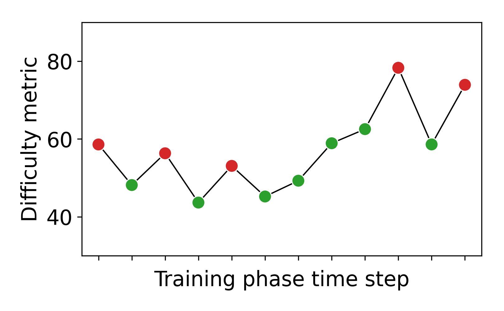
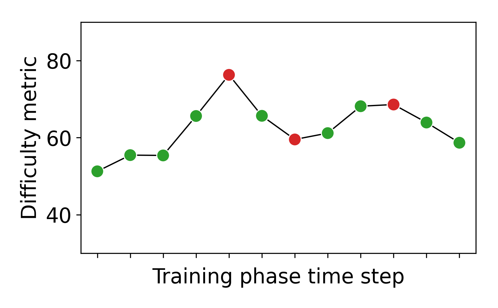
To get an in-depth view of how our algorithm performs, we show the progression of two individual participants in Figure 4. We list the training exercises they received and plot the difficulty of each exercise according to the handcrafted difficulty metric. Student A had the easy pre-test exercise correct and thus got assigned a medium exercise at first. In the beginning, it seems like they are staying in their zone of flow which can be seen by the zigzagging between slightly too easy and too hard exercises. Then they seem to improve which our algorithm picks up on and provides harder exercises. Towards the end, the adaptation again seems to reach the student’s flow zone. Student B also solved the easy pre-test correctly. After some successes, the DDA algorithm tried to give them a harder exercise but sees that the student could not work with it. After this, the difficulty stays quite level. Even when the student slips with exercises of a difficulty level they evidently solved before, the algorithm does not immediately decrease the difficulty. This seems to have been the correct procedure as student B stated in the post-questionnaire: “I felt like the difficulty level of the puzzle was just right as it made you think twice before answering.”.
© 2023 Copyright is held by the author(s). This work is distributed under the Creative Commons Attribution-NonCommercial-NoDerivatives 4.0 International (CC BY-NC-ND 4.0) license.