ABSTRACT
Predictive student models are increasingly used in learning
environments due to their ability to enhance educational
outcomes and support stakeholders in making informed
decisions. However, predictive models can be biased and
produce unfair outcomes, leading to potential discrimination
against some students and possible harmful long-term
implications. This has prompted research on fairness metrics
meant to capture and quantify such biases. Nonetheless, so far,
existing fairness metrics used in education are predictive
performance-oriented, focusing on assessing biased outcomes
across groups of students, without considering the behaviors of
the models nor the severity of the biases in the outcomes.
Therefore, we propose a novel metric, the Model Absolute
Density Distance (MADD), to analyze models’ discriminatory
behaviors independently from their predictive performance. We
also provide a complementary visualization-based analysis to
enable fine-grained human assessment of how the models
discriminate between groups of students. We evaluate our
approach on the common task of predicting student success in
online courses, using several common predictive classification
models on an open educational dataset. We also compare our
metric to the only predictive performance-oriented fairness
metric developed in education, ABROCA. Results on this
dataset show that: (1) fair predictive performance does not
guarantee fair models’ behaviors and thus fair outcomes,
(2) there is no direct relationship between data bias and
predictive performance bias nor discriminatory behaviors bias,
and (3) trained on the same data, models exhibit different
discriminatory behaviors, according to different sensitive
features too. We thus recommend using the MADD on models
that show satisfying predictive performance, to gain a
finer-grained understanding on how they behave and regarding
who and to refine models selection and their usage. Altogether,
this work contributes to advancing the research on fair student
models in education. Source code and data are in open access at
https://github.com/melinaverger/MADD.
Keywords
1. INTRODUCTION
Over the past decade, extensive research has focused on predictive student modeling for educational applications. The systematic literature review of Hellas et al. [15] has identified no less than 357 relevant papers on the matter published between 2010 and mid-2018. One of the most popular modeling technique in these works are machine learning (ML) classifiers, as many important predictive tasks in education can be framed as binary classification problems, e.g. to predict dropout, course completion, university admission, scholarship awarding. These classification models have thus gained widespread adoption, and the multiple stakeholders involved in education have recognized their potential to improve student learning outcomes and experience [29, 16].
However, in recent years, there have been concerns about the fairness of the models (also called algorithmic fairness [3]) used in education [3, 20, 11, 33]. This stems from a more general trend of research in ML and Artificial Intelligence (AI), where a large body of research has shown that classifiers, and AI models in general, can produce biased and unfair outcomes, e.g. [27, 5, 4, 23, 10]. This has led to increased public awareness about the potential harms of AI predictive models and the enforcement of stricter regulations1. In education too, recent studies have found that classification-based student models can be biased against certain groups of students, which could in turn significantly hinder their learning experience and academic achievements [3, 20, 33, 14, 17, 25].
To unveil, measure and mitigate algorithmic unfairness, recent literature in AI has seen a proliferation of fairness metrics [35, 7]. Although many types of metrics exist (see Section 2), some of them require extensive prior knowledge and in practice the most common fairness metrics used in AI are statistical [35]. Statistical metrics aim at quantifying the differences in performance of a set of classification models across different groups of interest, with the assumption that fair classifiers should achieve similar performance across groups [7]. This is especially meaningful when some of the groups are known to be vulnerable to unfair model predictions. For instance, students with disability might be unfairly classified as at-risk of dropping out of an online course because the features used to train the classifiers did not capture well the different way they engage with the learning material [13] – when they can interact at all, since many K-12 material or educational technologies remain inaccessible [31, 6]. Hovewer, the pitfall of the existing statistical metrics is that they are all predictive performance-oriented, meaning that they solely consider the predictive performance of the classification model across predefined groups, disregarding that two classifiers with equal predictive performance can exhibit very different, and possibly unfair, behaviors. In particular, a classifier could produce similar error rates across two groups, but the actual errors made could be substantially more harmful to one of the group than the other.
In this paper, we thus propose a new statistical metric, the Model Absolute Density Distance (MADD), to analyze a model’s discriminatory behaviors independently from its predictive performance. We also propose a complementary visualization-based analysis, which allows to inspect and qualify the models’ discriminatory behaviors uncovered by the MADD. Altogether, this makes it possible to not only quantify, but also understand in a fine-grained way whether and how a given classifier may behave differently between the groups. As a case study, we apply our approach on the common task of predicting student success to a course, on open data for the sake of replication and on four common predictive classification models for the sake of generalization. We also compare our metric to ABROCA (Absolute Between-ROC Area), the only predictive performance-oriented metric developed in education [14] to the best of our knowledge. This case study shows that the MADD can successfully capture fine-grained models’ discriminatory behaviors.
The remainder of this paper is organized as follows. Section 2 reports on related work on fairness metrics and their usage in education. Section 3 presents the MADD metric and the visualization-based analysis we propose to inspect and characterize models’ discriminatory behaviors. Section 4 describes the experimental setup with which we applied our proposed approach in order to demonstrate its benefits. Section 5 presents our results and our comparison with ABROCA. In Section 6, we discuss more generally what our approach allows to unveil, the strengths and limitations it currently has as well as some practical guidelines, before concluding in Section 7 with future work.
2. RELATED WORK
Several fairness metrics have been proposed in AI for classification models. These metrics mostly fall into three categories: counterfactual (or causality-based), similarity-based (or individual), and statistical (or group) [35]. The first two categories, counterfactual and similarity-based, are seldom used in practice because they require extensive prior knowledge. More precisely, counterfactual metrics require building a directed acyclic causal graph with the nodes representing the features of an applicant and the edges representing relationships between the features [35]. Generating such a causal graph is typically not feasible without extensive studies to formally identify these relations. Similarity-based metrics require defining a priori a distance metric to measure how “similar” two individuals are, as well as to know from which value the models’ results are considered “dissimilar” enough for these two individuals to be pointed out as unfairness. In contrast, statistical metrics, the category into which MADD falls, are easier to implement and more popular, as they solely require to identify a priori the groups of persons who might suffer from unfair classifications. As noted in the introduction, these metrics have so far sought to quantify differences in classification performance across the groups, and thus can be considered predictive performance-oriented only. However, a classifier that has similar error rates across two groups might actually produce errors that are harmless to a group but very harmful to the other, an aspect that is not quantified by existing statistical metrics. In this paper, we focus on the new MADD metric meant to assess unfair behaviors of classifiers, independently from their predictive performance. We recommend using it as a complement to a predictive performance analysis, rather than using predictive performance-oriented fairness metrics only, in order to gain a more refined and comprehensive understanding of the classifiers fairness.
In education, fairness studies are more recent and sparse (see overview in [3, 20]), and only a handful of them have focused on the fairness of classification models used in this context [14, 17, 18, 30, 25]. In Gardner et al. [14], the authors propose a new predictive performance-oriented fairness metric based on the comparison of the Areas Under the Curve (AUC) of a given predictive model for different groups of students. They used their metric to assess gender-based (male vs. female) differences in classification performance of MOOC dropout models, showing that ABROCA can capture unfair classification performance related to the gender imbalance in the data. ABROCA was also used in other educational studies, to evaluate the fairness across different sociodemographic groups of classifiers meant to predict college graduation [18], and categorize students’ educational forum posts [30]. The other fairness studies in education have used more common statistical metrics in AI, such as group fairness, equalized odds, equal opportunity, true positive rate and false positive rate between groups, to predict course completion [26], at-risk students [17], and college grades and success [19, 36, 25]. Similarly to ABROCA, these metrics are predictive performance-oriented. In this paper, we contribute to this line of fairness work in education by investigating the possibility and value of a fairness metric that accounts for the behaviors of the classifiers.
3. AN ALGORITHMIC FAIRNESS ANALYSIS APPROACH
3.1 Definition of the MADD metric
We introduce a novel metric, the Model Absolute Density Distance (MADD), which is based on measuring algorithmic fairness via models’ behavior differences between two groups, instead of via models’ predictive performance. It is worth noting that this focus on the models’ behaviors enables us to not only quantify algorithmic fairness, but also gain a deeper understanding of how the models discriminate via graphical representations of the MADD (see next subsection 3.2).
We present the MADD under the scope of this study where we consider binary sensitive features and binary classifiers that output probability estimates (or confidence scores) associated to their predictions.
Assume a model \(\mathcal {M}\), trained on a dataset \(\left \{ X, S, Y \right \}_{i = 1}^{n}\) where \(S\) are the binary sensitive features, \(X\) all the other features characterizing the students, \(Y \in \left \{ 0, 1 \right \}\) the binary target variable, and \(n\) the number of samples. \(\left \{ X, S \right \}_{i = 1}^{n}\) represents all the features of the prediction task. More precisely, \(S = (s_i^a)_{i=1}^n\) where \(a\) is the index of the considered sensitive feature and \(s_i^a \in \left \{ 0, 1 \right \} \). Indeed, if a student \( (x_i, s_i^a) \) belongs to any group named \(G_0\) of the sensitive feature \(a\), then \(s_i^a = 0\), and idem \(s_i^a = 1\) if \( (x_i, s_i^a) \) belongs to the other group named \(G_1\) of the same sensitive feature \(a\). Note that a sample \( (x_i, s_i^a) \) describes a unique student in a group, with the groups \(G_0\) and \(G_1\) being mutually exclusive (i.e. a student can only belongs to one of these two groups). Also, none of these groups is considered as a baseline or privileged group here.
\(\mathcal {M}\) aims at minimizing some loss function \(\mathcal {L}(Y, \hat {Y})\) with its predictions \(\hat {Y}\) to estimate or predict \(Y\). \(\mathcal {M}\) should assign to each \(\hat {Y}_i\) a predicted probability (or a confidence score) that a given sample \( (x_i, s_i^a) \) will be predicted as \(\hat {Y}_i = 1\). This probability or score is noted \(\hat {p}(x_i, s_i^a) = \mathrm {P} ( Y = 1 | X_i = x_i, S =s_i^a)\). We introduce a parameter \(e\) that is the probability sampling step of \(\hat {p}\) values between 0 and 1. In other words, \(\hat {p}\) values are rounded to the nearest \(e\) (e.g. \(\hat {p}(x_i, s_i^a) = 0.09\) if \(e = 0.01\) and the same \(\hat {p}(x_i, s_i^a) = 0.1\) if \(e = 0.1\) for instance). \(\mathcal {M}\) predicts \(\hat {Y}_i = 1\) if and only if \(\hat {p}(x_i, s_i^a) \geq t\) where \(t\) is a probability threshold, and \(\hat {Y}_i = 0\) otherwise.
We define two unidimensional vectors \(D_{G_0}^a\) and \(D_{G_1}^a\) as what we call in short the density vectors of the respective groups \(G_0\) and \(G_1\) of the sensitive feature \(a\). They actually contain all the density values associated to each \(\hat {p}(x_i, s_i^a)\) value (rounded to the nearest \(e\)) of group \(G_0\) or group \(G_1\). In particular, \(D_{G_0}^a = (d_{G_0,k}^a)_{k=0}^m\) where each \(d_{G_0,k}^a\) is the density of \(\hat {p}(x_i, s_i^a) = k \times e\) value, that is to say the frequency that the model \(\mathcal {M}\) gives \(\hat {p}(x_i, s_i^a) = k \times e\) divided by the sum of frequency of all \(\hat {p}\) values. \(m\) is equal to the total number of distinct \(\hat {p}\) values and is related to \(e\) by the following: \(m = 1/e + 1\). The advantage of the introduction of \(e\) could be seen here: having discretized the \(\hat {p}\) values enables us to have the two density vectors \(D_{G_0}^a\) and \(D_{G_1}^a\) of the same length so that they are comparable on the probability space and independent from the model \(\mathcal {M}\)’s behaviors.
We now define the MADD as follows: \begin {equation} \text {MADD}(D_{G_0}^a, D_{G_1}^a) = \sum _{k=0}^m | d_{G_0,k}^a - d_{G_1,k}^a | \label {MADDeq} \end {equation} The MADD satisfies the necessary properties of a metric: reflexivity, non-negativity, commutativity, and triangle inequality [9] (see the proofs in Appendix A). Moreover: \begin {equation} \forall a, \hspace {0.2cm} 0 \leq \text {MADD}(D_{G_0}^a, D_{G_1}^a) \leq 2 \label {MADDeq-boundaries} \end {equation}
The closer the MADD is to 0, the fairer the outcome of the model is regarding the two groups. Indeed, if the model produces the same probability outcomes for both groups, then \(D_{G_0}^a = D_{G_1}^a\) and \(\text {MADD}(D_{G_0}^a, D_{G_0}^a) = 0\). Conversely, in the most unfair case, where the model produces totally distinct probability outcomes for both groups, the MADD is equal to 2. An example of such a situation is when \(\exists k_{G_0}, d_{G_0,k_{G_0}}^a = 1\) and \(\forall k \in [0,m], k \neq k_{G_0}, d_{G_0,k}^a = 0\), and \(\exists k_{G_1} \neq k_{G_0}, d_{G_1,k_{G_1}}^a = 1\) and \(\forall k \in [0,m], k \neq k_{G_1}, d_{G_1,k}^a = 0\). In that case, Equation 1 becomes: \begin {equation} \text {MADD}(D_{G_0}^a, D_{G_1}^a) = | d_{G_0,k_{G_0}}^a| + | d_{G_1,k_{G_1}}^a| = (1 + 1) = 2 \end {equation}
3.2 Visualization-based analysis of models’ discriminatory behaviors
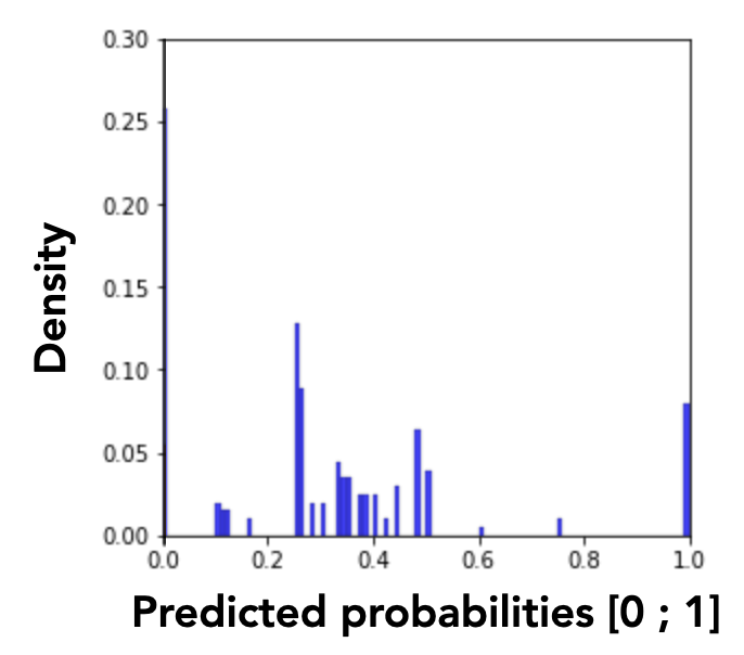
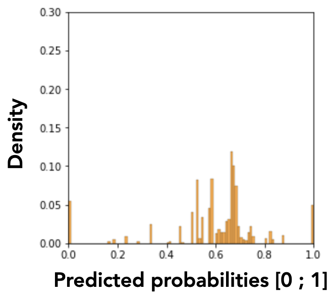
We introduce a visualization-based analysis of the models’ discriminatory behaviors that complements our fairness analysis approach. This analysis is based on graphical interpretations of the MADD. Let us plot in Figures 1a and 1b the density histograms associated with each density vector \(D_{G_0}^a\) and \(D_{G_1}^a\). These histograms represent the distributions of the \(\hat {p}\) values for the group \(G_0\) and the group \(G_1\) of a sensitive feature \(a\). The number and consequently the width of the intervals depend on the probability sampling step \(e\).
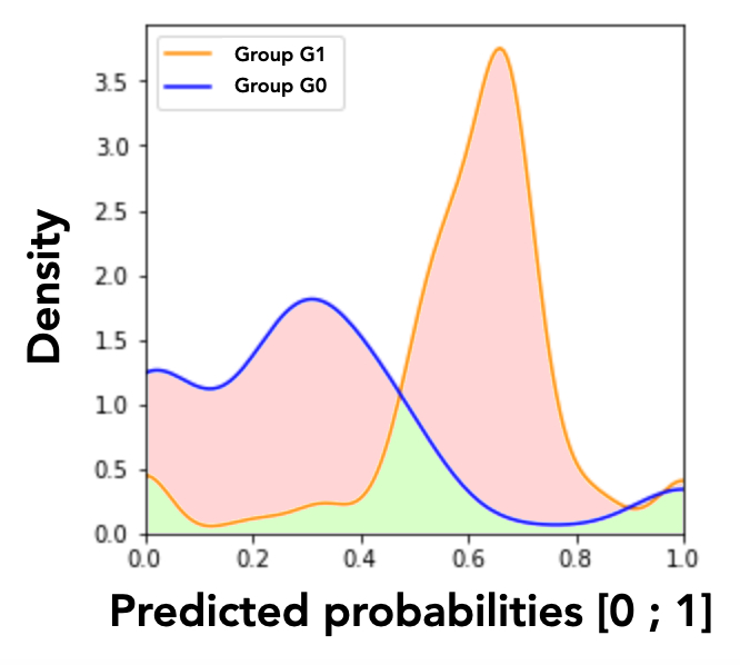
However, these histograms are not easily interpretable because of the numerous variations of the discrete values. We solve this issue by applying a smoothing by kernel density estimation (KDE) with Gaussian kernels, as shown in Figure 1c. The smoothing parameter, also called bandwidth parameter, is determined by the Scott’s rule, an automatic bandwidth selection method2. This smoothing transforms the discrete probability distribution (whose density values cannot exceed 1 in the y-axis as they are related to discrete random variables) into a continuous approximation of the associated probability density function (PDF), which can in turn take values greater than 1.
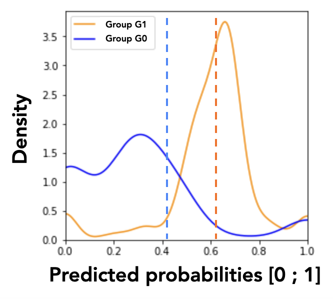
Therefore, a visual approximation of the MADD corresponds to the red area in Figure 1d. Indeed, as the MADD uses the absolute density distances point-by-point between the two density vectors, the metric can be visually approximated by the area in-between the two curves, considering that the graph shows continuous density instead of the true discrete values used in the MADD calculation. Conversely, the green area, which is the intersection of the smoothed representations of the two density vectors, illustrates the area where the model \(\mathcal {M}\) produces the same predicted probabilities for both groups up to a certain approximated density. We call this area the fair zone.

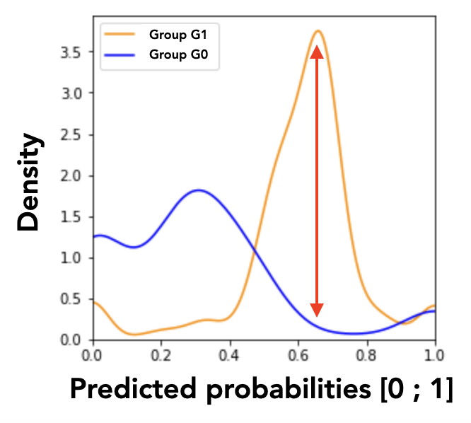
Thanks to this graphical representation approximating the MADD, we are able to distinguish two model’s discriminatory behaviors: unequal treatment (Figure 2a), and stereotypical judgement (Figure 2b). Unequal treatment behavior can be summarized as follows: “how much the model favor or penalize individuals based on them belonging to each group?” As displayed in Figure 2a, we can identify which group get lower or higher predicted probabilities on average, allowing us to understand which group the model tends to favor (the highest mean, here the group \(G_1\)) or to penalize (the lowest mean, here the group \(G_0\)). It is worth noticing that the means are not perfectly aligned with the peaks of the distributions because they are calculated from the density vectors, without the smoothing. The second discriminatory behavior, stereotypical judgement, can be summarized as follows: “how much the model makes repetitive and invariant “judgement” about the individuals based on them belonging to a group?” For instance in Figure 2b, the model clearly tends to give to many persons in the group \(G_1\) the same predicted probabilities. These analyses cannot be performed with existing predictive performance-oriented fairness metrics, as the model could have the same accuracy for both groups regardless of its underlying effective predictions, either in terms of distributions or in terms of density differences.
4. EXPERIMENTAL SETTING
We apply our approach on the common task of predicting student success to a course, and we present in this section (1) the data, (2) the models, and (3) the setting parameters we used in our experiments. This case study is designed to further investigate our proposed approach, and to show how one can use it.
4.1 Data
4.1.1 Dataset presentation
We used real-world anonymized data from the Open University Learning Analytics Dataset (OULAD) [22]. The Open University is a distance learning university from the United Kingdom, offering higher education courses which can be taken as standalone courses or as part of a university program with no previous qualifications required. The dataset contains both student demographic data and interaction data with the university’s virtual learning environment (VLE). The students were enrolled in at least one of the three courses in Social Sciences or one of the four Science, Technology, Engineering and Mathematics (STEM) courses between 2013 and 2014. The dataset contains 32,593 samples including 28,785 unique students.
The choice of this dataset was motivated by several reasons. First, the OULAD is one of the most comprehensive and benchmark datasets in the learning analytics domain to assess the performance of students in a VLE [1]. In addition, it is an open dataset that answers the call to the community for the development of new approaches on open datasets [15]. Then, it also answers another call from [15] for replication in multiple contexts such as several courses with diverse populations, as provided in the OULAD. Moreover, as it is commonly the case with distance learning universities, the students have a large variety of profiles [8] (including on average more women than men and a wide age range [2]), and these information are available in the dataset, making it particularly relevant for studying the impact of demographic features in terms of fairness. Finally, the data was collected in compliance with The Open University requirements regarding ethics and privacy, including consent and anonymization.
4.1.2 Data preprocessing
| Name | Feature type | Description |
|---|---|---|
gender | binary | the students’ gender |
age | ordinal | the interval of the students’ age |
disability | binary | indicates whether the students have declared a disability |
highest_education | ordinal | the highest student education level on entry to the course |
poverty3 | ordinal | specifies the Index of Multiple Deprivation [22] band of the place where the students lived during the course |
num_of_prev_attempts | numerical | the number of times the students have attempted the course |
studied_credits | numerical | the total number of credits for the course the students are currently studying |
sum_click | numerical | the total number of times the students interacted with the material of the course |
We used the features presented in Table 1. The sum_click
feature was the only one that was not immediately available in
the original dataset and was computed from inner joints and
aggregation on the original data. Also, we removed samples
where the value of the poverty feature was missing (4% of the
data samples) and when the students withdrew from the courses
(24% of the data samples). This left us with 19,964 samples of
distinct students, whose values were scaled between 0 and 1 for
every feature via normalization. We indeed did not apply
standardization to keep the original data distributions and
analyze the models’ behaviors accordingly. The target variable
(course outcome) was coded as “Pass” or “Fail” (1 or 0
respectively). Plus, students who got a “Distinction” outcome
were also coded as 1 (“Pass”), as we target binary classification
for this case study.
In our study, we considered three sensitive features: gender,
poverty, and disability. Although other sensitive features
could have been relevant, our main focus here is in investigating
our proposed method itself. Therefore, one may choose different
sensitive features according to their purpose (for instance
including age as well, as in [34]), and one would be able to
conduct the same fairness analysis process. Due to our
method dealing with binary features as sensitive features, we
transformed poverty into a binary feature by setting a 50%
threshold of deprivation index [22], coding as 0 those below the
50% threshold (i.e. less deprived) and as 1 those above (i.e.
more deprived).
We did not apply any data balancing techniques nor unfairness mitigation preprocessing, still to keep the original data distributions. However, our approach does not prevent the use of such preprocessing.
4.1.3 Data analyses and course selection
We explored the correlations and imbalances of the sensitive
features across the different courses in the dataset to identify
those which were relevant for analysing algorithmic fairness. We
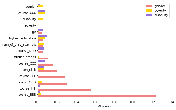
thus computed the mutual information (MI) between all the
features and the three sensitive ones, whose respective results
are distinguished by a different color as shown in Figure 3.
Mutual information is particularly relevant for non-linear
relationships between features. Figure 3 shows that the
course “BBB” followed by the course “FFF” are the most
correlated with the gender feature, with the overall highest
MI scores. Therefore, the Social Sciences course coded as
“BBB” and the STEM course coded as “FFF”, two different
student populations, were good candidates for examining the
impact of gender bias on the predictive models fairness. In
addition, both courses presented very high imbalances in
terms of disability (respectively 91.2-8.8% and 91.7-8.3%
for 0-1 groups in courses “BBB” and “FFF”) and gender
(respectively 88.4-11.6% and 17.8-82.2% for 0-1 groups
in courses “BBB” and “FFF”), and still some imbalance
for poverty (respectively 42.3-57.7% and 46.9-53.1% for 0-1 groups in courses “BBB” and “FFF”). Based on these
preliminary unfairness expectations derived from the skews in
the data, it is interesting to analyze whether and how
the models will suffer from these biases in both courses.
These two courses are thus excellent testbeds for testing our
approach.
4.2 Classification Models
To show that our fairness analysis approach can handle several types of classification models, we chose models either based on regression, distance, trees, or probabilities. More precisely, we chose a logistic regression classifier (LR), a k-nearest neighbors classifier (KN), a decision tree classifier (DT), and a naive bayes classifier (NB).
We chose these particular models for the following reasons. Firstly, they are widely used in education, and specially with the OULAD [21, 1]. Models based on vectors (e.g. support vector machines), also commonly used, were not selected as they do not outcome probability estimates (or confidence scores) on which to run our fairness analysis. Secondly, while our approach can be generalized to other models with probability estimates (or confidence scores) such as random forest or neural networks, we favored white boxes and explainability over finding the best modeling with fine-tuning. Thirdly, predicting students’ success with the data in the OULAD is a rather low abstraction task due to the small amount of features and variance in the data, for which using complex predictive models would not lead to better performance and could even overfit the data. Finally, the selected models are easy to implement for most use cases, which makes them universally good candidates for predictive modeling in general.
To fit the models, we split the data into a train and a test set using a 70-30% split ratio in a stratified way, meaning that we kept the same proportion of students who passed and failed in both the train and the test sets. The resulting accuracies of the models were above the baseline (70%) and up to 93%, except for the NB (62%) which instead presented interesting behaviors with the MADD analyses and was worth keeping it (see Section 5). It has to be noted that, contrary to most ML studies, achieving the best predictive performance was not our focus here, since the purpose of our experiments is rather to analyze the fairness of diverse models with the MADD metric. Then, we used the models’ outcomes on the test set to compute the MADD metric and generate the visualizations.
4.3 Fairness Parameters
For our study, we set \(e\) to 0.01 (i.e. \(m=101\)), and \(t\), the probability classification threshold, to 0.5. For \(e\), 0.01 corresponds to a variation of the probability of success or failure of 1%, which we deem a sufficient level of probability sampling precision, considering on the one hand that probability variations below 1% are not significant enough in the problem, and on the other hand that higher values of \(e\) (up to 0.1) did not alter the MADD results. Regarding \(t\), the success prediction is generally defined by having an average score above 50% and thus we chose \(t\) with respect to the problem rather than optimizing it for model performance. The odds of positive or negative predictions are thus balanced and the threshold is the same for each individual.
5. RESULTS
In the following, we show in subsection 5.1 how the MADD and its visualization-based analysis can help unveil unexpected results based on (1) the respective importance of each sensitive feature in algorithmic unfairness, (2) the models intrinsic unfairness, and (3) the nature of the unfairness associated with the predictions made by the model. Then, we show in subsection 5.2 how our results differ from and complement what can be provided by ABROCA, a state-of-the-art predictive performance-oriented fairness metric. Both subsections 5.1 and 5.2 are concluded by a summary of the obtained results.
5.1 Fairness Analysis with MADD
In the parts 5.1.1 and 5.1.2, we examine via Tables 2 and
3 the MADD results reported for the two courses. We
highlight in bold the best MADD per column, and with
an asterisk (*) the best MADD per row. In this way, the
MADD of the fairest model for each sensitive feature is in
bold, whereas the MADD of the fairest sensitive feature
for each classifier is marked with a *. As examples, in
Table 2 the DT is the fairest model regarding the poverty feature (bold), and in Table 3 the disability feature is
the fairest for the KN (*). For the part 5.1.3, we base
our visual analyses and identification of discriminatory
behaviors explained in subsection 3.2 on Figures 4 and
5.
5.1.1 Sensitive features analysis
Table 2 reveals that three models out of four (LR, KN, and DT)
are the fairest for the disability sensitive feature. Therefore,
two interesting observations can be made. First, it is contrary to
what we would expect since disability was the most
imbalanced (91.2-8.8% for 0-1 groups) sensitive feature in the
training data (see Section 4.1.3). Second, the gender feature
was particularly expected to be highly sensitive due to
its high correlation with the target in this course and its
imbalance, but it actually has the best MADD on average
(1.02).
Similarly to the above results for the course “BBB”, we can
notice that the data skews are not necessarily reflected in the
MADDs. In the training data, the disability sensitive feature
was highly imbalanced, and the poverty feature was quite
balanced. Nonetheless, for half of the models (see Table 3), both
disability and poverty are the two sensitive features with
regard to which the models are the fairest. On the other
hand, in line with the gender skew and correlation shown
in Section 4.1.3, gender has the worst MADD results in
average, more than disability, although the difference is not
substantial.
5.1.2 Model fairness analysis
Now focusing on the fairness of the models, DT appears in
Table 2 to be the fairest, with an average MADD of 0.73
across all the sensitive features. DT is indeed the fairest for
disability and poverty and the second best for gender. On
the contrary, LR is the least fair, with the highest results for
each senstive feature and an average of 1.71, with a maximum
value of 2.
NB and DT obtain the best
MADD averages across all three sensitive features (0.64 and
0.65 respectively). Therefore, there is no clear winner for this
course as they behave differently according to different sensitive
features: NB has better results for gender and poverty but a
higher MADD for disability, whereas DT is more balanced
across the three sensitive features. However, we remind that NB
performed below the accuracy baseline and thus DT would
overall be a better candidate.
Model | Sensitive features | ||||
|---|---|---|---|---|---|
gender | poverty | disability | Average | ||
MADD | LR | 1.72 | 1.85 | 1.57* | 1.71 |
| KN | 1.13 | 1.12 | 0.93* | 1.06 | |
| DT | 0.69 | 0.85 | 0.65* | 0.73 | |
| NB | 0.52* | 0.9 | 1.37 | 0.93 | |
| Average | 1.02 | 1.18 | 1.13 | ||
Model | Sensitive features | ||||
|---|---|---|---|---|---|
gender | poverty | disability | Average | ||
MADD | LR | 1.18 | 1.06* | 1.12 | 1.12 |
| KN | 1.06 | 0.93 | 0.78* | 0.92 | |
| DT | 0.76 | 0.65 | 0.55* | 0.65 | |
| NB | 0.56 | 0.47* | 0.90 | 0.64 | |
| Average | 0.89 | 0.78 | 0.84 | ||
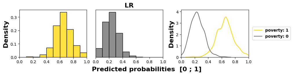
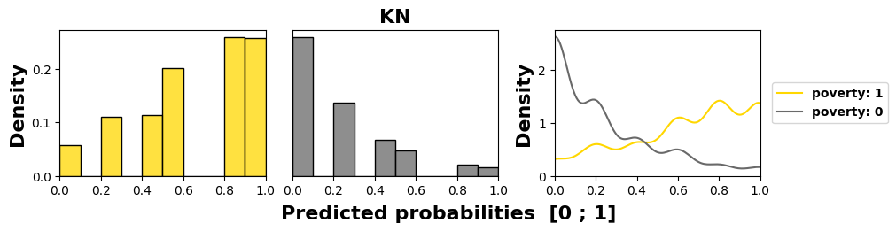
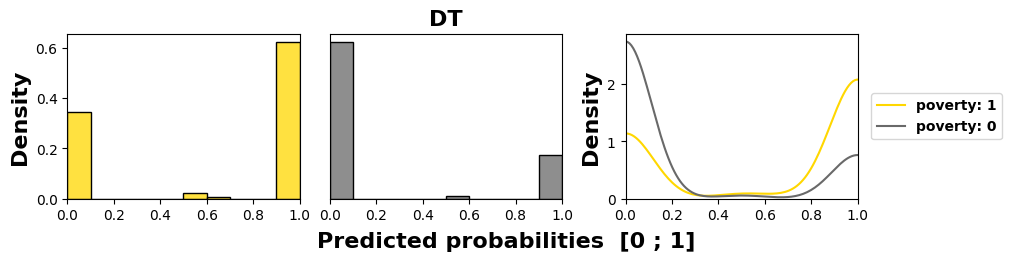
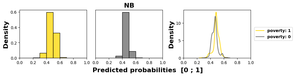
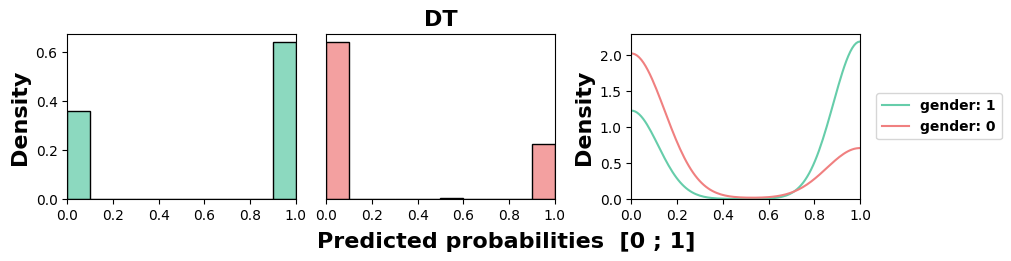
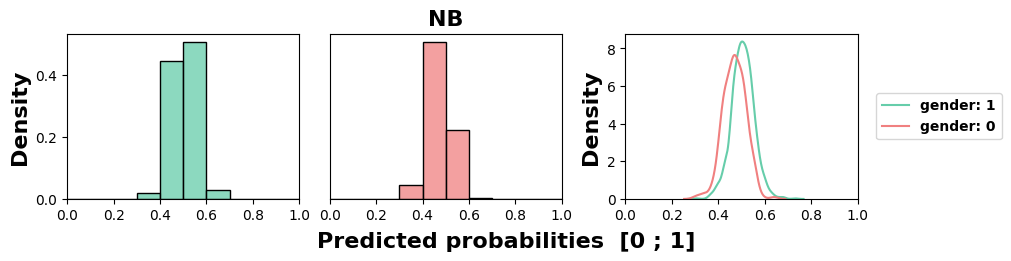
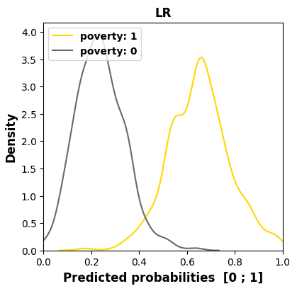
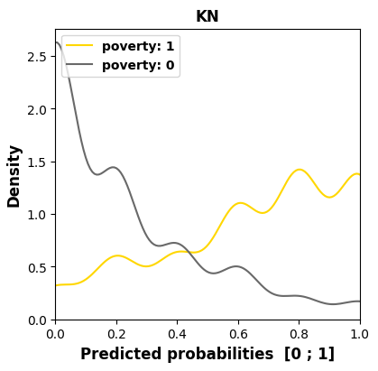
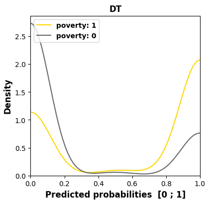
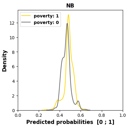
5.1.3 Visualization-based analysis
We examine in Figure 4 the models’ behaviors regarding the
most sensitive feature, namely poverty in this course, as it has
the worst MADD on average (1.18). We see in the subfigures,
through an offset of the distribution mean to the left for the
group 0, that three models out of four (LR, KN, and DT)
have learned unequal treatment against those in better
financial conditions (group 0). Among them, KN and DT
present the highest stereotypical results reduced to only few
probability values, which illustrates well their inner workings.
Conversely, NB produces the least discriminating results with
the closest means for the two groups. Its behavior is all the
more interesting since it shows that having poor predictive
performance is not necessarily interfering with behaving
fairly regarding two groups of the most sensitive feature. It
is precisely because it does not discriminate against any
features, whether they were sensitive or not, that it has poor
accuracy.
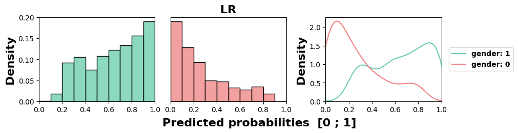
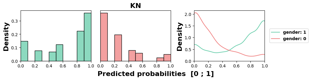
Likewise, we examine in Figure 5 the models’ behaviors for the
most sensitive feature in this course, gender, with the worst
MADD average of 0.89. All models but NB exhibit unequal
treatment against group 0, here the women. Similarly to the
previous results, we can again note the highly stereotypical
behaviors of KN and DT, and the relative fairness of the NB
model.
5.1.4 Implications for the MADD
Following the double reading of the tables, feature-wise or model-wise, as well as our visual analyses, we can make two important observations regarding the insights provided by the MADD.
Firstly, there is no direct relationships between biases in the data (imbalanced representations, high correlations) and the discriminatory behaviors learned by the models. We even observe opposite conclusions (specially for the course “BBB” in part 5.1.1).
Secondly, trained on the same data, the models exhibit very different discriminatory behaviors (see parts 5.1.2 and 5.1.3), both regarding different sensitive features, and different severity and nature of their algorithmic unfairness. This was also shown by our visual analysis, which allowed finer-grained interpretations of the discriminatory behaviors.
5.2 Comparison with ABROCA
We now aim to compare the MADD with the ABROCA predictive performance-oriented fairness metric [14]. The ABROCA results (computed with the source code from [12]) are displayed in Tables 4 and 5, and an illustrated example for the course “BBB” is given through the Figures 6 and 7.
5.2.1 Sensitive features analysis
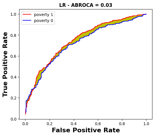
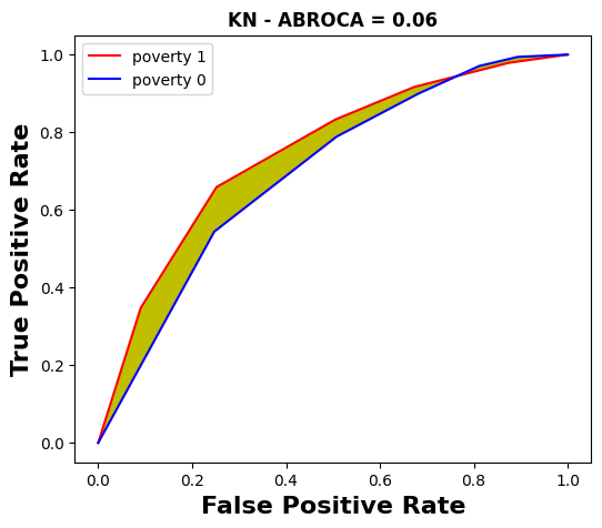
Let us first focus on the poverty feature which has the
worst MADD average (1.18 from Table 2). In particular, in
part 5.1.1, poverty was the feature with which LR obtained the
worst MADD (1.85 from Table 2), which was also the worst
MADD overall. Indeed, in Figure 6 it can be seen that LR has
the smallest intersection area compared to the other models.
However, in Figure 7 and Table 4 we see that LR has one of
the best ABROCA (0.03) with minimal area between the curves
of the respective groups. We found similar opposite results
between MADD and ABROCA for gender. Thus, poverty
and gender could be seen as unfair sensitive features for
a model on the one hand (MADD) and as fair ones on
the other hand (ABROCA). Moreover, DT too has one
of the best ABROCA (0.03), while it provided the best
MADD value (0.85 from Table 2) regarding this feature.
Therefore, two models with the same ABROCA lead to opposite
discriminatory behaviors according to the MADD. In the
end, ABROCA and MADD do not highlight the same
fairness results, and can even lead them to show opposite
results.
Now examining Table 5 for the course “FFF”, ABROCA does
not capture substantial differences at the sensitive feature level
(column-wise), with an ABROCA average of 0.4 for all three
features. Thus, the MADD results can capture additional
differences among the models’ behaviors that are not reflected
in the ABROCA results. In addition, we again found that
disability, the most imbalanced sensitive feature, is actually
the feature for which DT is the fairest, regardless of whether we
consider the MADD in part 5.1.1 (Table 3) or the ABROCA
(Table 5). Therefore, ABROCA does not reflect the imbalance
bias in the data either, in contradiction with the findings from
[14].
poverty sensitive feature across all the models for course “BBB”.
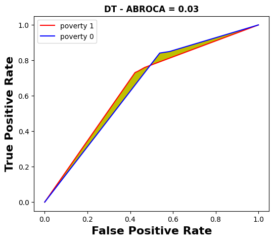
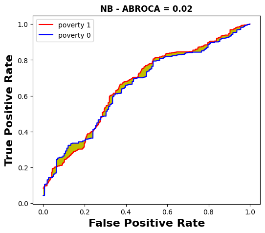
poverty sensitive feature across all the models for course “BBB”.
5.2.2 Model fairness analysis
In Table 4, LR and NB appear to be the fairest models across all the sensitive features (best common ABROCA average of 0.3). However, with the MADD, NB indeed exhibited overall quite balanced low values, but LR was always the least fair on average (Tables 2 and 3). Thus, at the model level this time, the trends in the MADD results are only partially reflected in the ABROCA results.
Table 5 shows that ABROCA results do not exhibit substantial
variability to distinguish differences in fairness between
the models (row-wise this time) in our experiment. In
addition to similar ABROCA averages, all models have very
close ABROCA results specially regarding the gender and
poverty features. Therefore, the MADD allows to find
complementary discriminatory results as compared to using only
ABROCA.
5.2.3 Summary of the comparison
Two main takeaways could be reported from our comparison between the ABROCA and MADD metrics.
Firstly, fair predictive performance (i.e. similar numbers of errors across groups, here captured by low ABROCA values) does not guarantee fair models’ behaviors (i.e. low severity of discrimination across groups, here captured by low MADD values). This demonstrates what we advocated in the introduction (Section 1) regarding investigating the models’ behaviors to gain a comprehensive understanding of the models fairness. In particular, two models with the same ABROCA could suffer from substantial, and even opposite algorithmic discriminatory behaviors, which can be uncovered by the MADD (see parts 5.2.1 and 5.2.2). Using the MADD together with a predictive performance-oriented metric such as ABROCA can thus allow more informed selection of fair models in education, and here in our experiments, they provide strong evidence that DT is the fairest model on both courses.
Secondly, in line with our previous findings that biases in the data may not be related with models’ discriminatory behaviors (see part 5.1.4), we also observed that the biases in the data are independent from predictive performance biases too. For instance, the highest imbalanced sensitive feature could actually lead to both the best ABROCA and the best MADD. Although this observation is aligned with the findings in [11, 17], it is worth noting that it goes against what the authors of ABROCA had observed [14] (see part 5.2.1).
Model | Sensitive features | ||||
|---|---|---|---|---|---|
gender | poverty | disability | Average | ||
ABROCA | LR | 0.02 | 0.03 | 0.03 | 0.03 |
| KN | 0.08 | 0.06 | 0.06 | 0.07 | |
| DT | 0.06 | 0.03 | 0.05 | 0.05 | |
| NB | 0.04 | 0.02 | 0.04 | 0.03 | |
| Average | 0.05 | 0.04 | 0.05 | ||
Model | Sensitive features | ||||
|---|---|---|---|---|---|
gender | poverty | disability | Average | ||
ABROCA | LR | 0.04 | 0.03 | 0.03 | 0.03 |
| KN | 0.04 | 0.05 | 0.04 | 0.04 | |
| DT | 0.05 | 0.04 | 0.01 | 0.03 | |
| NB | 0.03 | 0.03 | 0.07 | 0.04 | |
| Average | 0.04 | 0.04 | 0.04 | ||
6. DISCUSSION
In this section, we discuss (1) the overall implications of the results of our fairness study, (2) the limitations and the strengths of the proposed approach, (3) some potential experimental improvements, and (4) some guidelines to use our fairness analysis approach with the MADD.
6.1 Fairness results
Our results lead to three main conclusions, as follows. Firstly, we found no direct relationships between data bias and predictive performance bias nor discriminatory behaviors bias. It confirms previous findings that unfair biases are not only captured in the data, but are inherent to the model too [27, 28]. It further suggests that exclusively mitigating unfairness in the data might not be sufficient, and that mitigating unfairness at the model level is key too. Secondly, even trained on the same data, each model exhibits its own discriminatory behavior (likely linked to its inner working) and according to different sensitive features. It raises interesting questions on how different models could be combined in order to balance discriminatory behaviors with regards to multiple sensitive features at the same time. Thirdly, fair predictive performance does not guarantee by itself fair models’ behaviors and thus fair outcomes. Additional introspection of the model is therefore needed, and our approach appears as a possible solution.
6.2 Limitations and strengths
Although our approach was initially designed for analyzing algorithmic fairness at an individual sensitive feature level, our prospective work includes a generalization of the MADD metric to capture the influence of multiple sensitive features simultaneously. Moreover, the current MADD is particularly suitable for binary sensitive features and binary classifiers, and future work should also focus on extending it to multi-class features and classifiers. As an example, an extension for categorical sensitive features would enable us to have a finer-grained analysis of discrimination across more relevant subgroups. Despite these current limitations, the strengths of our approach stand in (1) its ability to be used with any tabular data, the most prevalent data representation [24] from any domain, and without needing any unfairness mitigation preprocessing; (2) being able to have a richer understanding of models’ discriminatory behaviors and their quantification with an easy-to-implement fairness metric that is independent from predictive performance; and (3) since the MADD is bounded, being comparable between different datasets to measure the discriminatory influence of a particular sensitive feature in different contexts and populations.
6.3 Experimental improvements
In our experiments we purposely focused on the MADD results to highlight its contribution and interest to fairness analysis, however for real-case applications one should obviously pay attention to both predictive performance and fairness performance in order to thoroughly select satisfying models. As an example, the NB model used in our experiments could be seen as fair regarding its MADD results, but it had in fact poor accuracy particularly because it was unable to predict well the success or the failure of students regarding any features, which makes this model not usable for real-case purposes but nonetheless interesting for our exploratory analysis. We thus recommend using the MADD on models that show satisfying predictive performance, to gain a finer-grained understanding on how they behave and regarding who and to refine models selection and their usage. Moreover, one should also consider testing variations of the probability sampling parameter \(e\) in their application and context. Although the impact of its variation in the range from 0.01 to 0.1 was low in our experiments, it might not be always the case. Determining the optimal value for this parameter is also a key part of our prospective work. Finally, we have demonstrated the validity and value of our approach on two courses of the OULAD dataset. Nonetheless, in a broader context of investigating model unfairness, this work should be replicated with other educational datasets providing more students data and more diverse sensitive features [3].
6.4 Guidelines
In order to facilitate replication studies and the use of our approach (in addition to the availability of the data and our source code), we provide in the following a 7-step guide to help readers compute the MADD and plot the models’ behaviors as in Figures 4 and 5.
- 1.
- Choose binary classification models that can output probability estimates or confidence scores.
- 2.
- Transform, when needed, every sensitive feature into binary one.
- 3.
- Train the models, and in the testing phase separate their predicted probabilities or confidence scores according to the groups of each sensitive feature.
- 4.
- Compute the MADD for each sensitive feature, and compare the results between features and models.
- 5.
- Plot histograms of the predicted probability distributions of each group of the sensitive features, and their smoothed estimations (e.g. with KDE).
- 6.
- Visually identify discriminatory behaviors among unequal treatment (i.e. distance between the two distribution means) and stereotypical judgement (i.e. differences of local amplitudes).
- 7.
- Depending on the fairness analysis goals:
- Identify which models are the fairest overall or according to which sensitive features, using a row-wise reading of the results table.
- Identify which features are the most sensitive overall or according to which models, using a column-wise reading of the results table.
- Using the plots, identify which groups (i.e. which distributions) are the most discriminated against by the models (relatively to each sensitive feature).
7. CONCLUSION
In this paper, we developed an algorithmic fairness analysis approach based on a novel metric, the Model Absolute Density Distance (MADD). It measures models’ discriminatory behaviors between groups, independently from their predictive performance. Our results on the OULAD dataset and comparison with ABROCA show that (1) fair predictive performance does not guarantee fair models’ behaviors and thus fair outcomes, (2) there is no direct relationships between data bias and predictive performance bias nor discriminatory behaviors’ bias, and (3) trained on the same data, models exhibit different discriminatory behaviors and according to different sensitive features.
This approach, for which we provide a set of guidelines in
subsection 6.4 and our source code and data in open access at
https://github.com/melinaverger/MADD, can be used to help
identify fair models, exhibit sensitive features, and determine
students who were the most discriminated against and how
(unequal treatment or stereotypical judgement) in an education
context. Being bounded, an advantage of this metric is
that it can be used across different contexts and data to
discover the features that more generally cause algorithmic
discrimination.
Future work will involve the generalization of the MADD metric to multiple sensitive features, its extension to multi-class sensitive features and classifiers, determining the optimal probability sampling parameter, and we will investigate how to use the MADD as an objective function to optimize models accordingly (in addition to predictive performance objectives).
8. ACKNOWLEDGMENTS
The authors want to thank Chunyang Fan (Sorbonne Université) for his valuable comments on this work.
9. REFERENCES
- H. A. Alhakbani and F. M. Alnassar. Open Learning Analytics: A Systematic Review of Benchmark Studies using Open University Learning Analytics Dataset (OULAD). In 2022 7th International Conference on Machine Learning Technologies (ICMLT), ICMLT 2022, pages 81–86, New York, NY, USA, June 2022. Association for Computing Machinery.
- C. B. Aslanian and D. L. Clinefelter. Online college students 2012. The Learning House, Inc. and EducationDynamics, 2012.
- R. S. Baker and A. Hawn. Algorithmic Bias in Education. International Journal of Artificial Intelligence in Education, 32:1052–1092, Nov. 2021.
- T. Bolukbasi, K.-W. Chang, J. Zou, V. Saligrama, and A. Kalai. Man is to Computer Programmer as Woman is to Homemaker? Debiasing Word Embeddings. In 30th Conference on Neural Information Processing Systems (NIPS 2016), pages 4349–4357, July 2016.
- J. Buolamwini and T. Gebru. Gender Shades: Intersectional Accuracy Disparities in Commercial Gender Classification. In Proceedings of the 1st Conference on Fairness, Accountability and Transparency, pages 77–91. PMLR, Jan. 2018. ISSN: 2640-3498.
- S. Burgstahler. Opening Doors or Slamming Them Shut? Online Learning Practices and Students with Disabilities. Social Inclusion, 3(6):69–79, Dec. 2015.
- A. Castelnovo, R. Crupi, G. Greco, D. Regoli, I. G. Penco, and A. C. Cosentini. A clarification of the nuances in the fairness metrics landscape. Scientific Reports, 12(1):1–21, 2022.
- J. Castles. Persistence and the adult learner: Factors affecting persistence in open university students. Active Learning in Higher Education, 5(2):166–179, 2004.
- S.-H. Cha and S. N. Srihari. On measuring the distance between histograms. Pattern Recognition, 35:1355–1370, 2002.
- J. Dastin. Amazon scraps secret AI recruiting tool that showed bias against women, Oct 2018. Reuters.
- O. B. Deho, C. Zhan, J. Li, J. Liu, L. Liu, and T. Duy Le. How do the existing fairness metrics and unfairness mitigation algorithms contribute to ethical learning analytics? British Journal of Educational Technology, 53(4):822–843, 2022.
- V. Disha. https://pypi.org/project/abroca (v. 0.1.3).
- L. Foreman-Murray, S. Krowka, and C. E. Majeika. A systematic review of the literature related to dropout for students with disabilities. Preventing School Failure: Alternative Education for Children and Youth, 66(3):228–237, July 2022.
- J. Gardner, C. Brooks, and R. Baker. Evaluating the Fairness of Predictive Student Models Through Slicing Analysis. In Proceedings of the 9th International Conference on Learning Analytics & Knowledge, pages 225–234, Tempe AZ USA, Mar. 2019. ACM.
- A. Hellas, P. Ihantola, A. Petersen, V. V. Ajanovski, M. Gutica, T. Hynninen, A. Knutas, J. Leinonen, C. Messom, and S. N. Liao. Predicting academic performance: A systematic literature review. In Proceedings Companion of the 23rd Annual ACM Conference on Innovation and Technology in Computer Science Education, ITiCSE 2018 Companion, page 175–199, New York, NY, USA, 2018. Association for Computing Machinery.
- K. Holstein and S. Doroudi. Equity and Artificial Intelligence in Education: Will “AIEd" Amplify or Alleviate Inequities in Education? arXiv:2104.12920, 2021.
- Q. Hu and H. Rangwala. Towards Fair Educational Data Mining: A Case Study on Detecting At-risk Students. Proceedings of The 13th International Conference on Educational Data Mining (EDM 2020), page 7, 2020.
- S. Hutt, M. Gardner, A. L. Duckworth, and S. K. D’Mello. Evaluating fairness and generalizability in models predicting on-time graduation from college applications. International Educational Data Mining Society, 2019.
- W. Jiang and Z. A. Pardos. Towards equity and algorithmic fairness in student grade prediction. In Proceedings of the 2021 AAAI/ACM Conference on AI, Ethics, and Society, pages 608–617, 2021.
- R. F. Kizilcec and H. Lee. Algorithmic Fairness in Education. arXiv:2007.05443 [cs], Apr. 2021.
- C. Korkmaz and A.-P. Correia. A review of research on machine learning in educational technology. Educational Media International, 56(3):250–267, 2019.
- J. Kuzilek, M. Hlosta, and Z. Zdrahal. Open university learning analytics dataset. Sci Data 4, 170171, 2017.
- J. Larson, S. Mattu, L. Kirchner, and J. Angwin. How We Analyzed the COMPAS Recidivism Algorithm. ProPublica, 2016.
- T. Le Quy, A. Roy, V. Iosifidis, W. Zhang, and E. Ntoutsi. A survey on datasets for fairness-aware machine learning. WIREs Data Mining and Knowledge Discovery, 12(3):e1452, 2022.
- H. Lee and R. F. Kizilcec. Evaluation of Fairness Trade-offs in Predicting Student Success. arXiv:2007.00088 [cs], June 2020.
- C. Li, W. Xing, and W. Leite. Yet another predictive model? Fair predictions of students’ learning outcomes in an online math learning platform. In Proceedings of the 11th International Learning Analytics and Knowledge Conference, pages 572–578, 2021.
- N. Mehrabi, F. Morstatter, N. Saxena, K. Lerman, and A. Galstyan. A Survey on Bias and Fairness in Machine Learning. arXiv:1908.09635 [cs], Jan. 2022. arXiv: 1908.09635.
- D. Pessach and E. Shmueli. Algorithmic Fairness. arXiv:2001.09784 [cs, stat], Jan. 2020.
- C. Romero and S. Ventura. Educational data mining and learning analytics: An updated survey. Wiley Interdisciplinary Reviews: Data Mining and Knowledge Discovery, 10:e1355, 2020.
- L. Sha, M. Rakovic, A. Whitelock-Wainwright, D. Carroll, V. M. Yew, D. Gasevic, and G. Chen. Assessing algorithmic fairness in automatic classifiers of educational forum posts. In International conference on artificial intelligence in education, pages 381–394. Springer, 2021.
- N. L. Shaheen and J. Lazar. K-12 Technology Accessibility: The Message from State Governments. Journal of Special Education Technology, 33(2):83–97, June 2018.
- F. Sovrano, S. Sapienza, M. Palmirani, and F. Vitali. A Survey on Methods and Metrics for the Assessment of Explainability under the Proposed AI Act. In Legal Knowledge and Information Systems: JURIX 2021: The Thirty-fourth Annual Conference, volume IOS Press, pages 235–242, Vilnius, Lithuania, 2022.
- J. Vasquez Verdugo, X. Gitiaux, C. Ortega, and H. Rangwala. FairEd: A Systematic Fairness Analysis Approach Applied in a Higher Educational Context. In LAK22: 12th International Learning Analytics and Knowledge Conference, pages 271–281, Online USA, Mar. 2022. ACM.
- M. Verger, F. Bouchet, S. Lallé, and V. Luengo. Caractérisation et mesure des discriminations algorithmiques dans la prédiction de la réussite à des cours en ligne. In 11ème Conférence sur les Environnements Informatiques pour l’Apprentissage Humain (EIAH 2023), Brest, France, June 2023.
- S. Verma and J. S. Rubin. Fairness definitions explained. 2018 IEEE/ACM International Workshop on Software Fairness (FairWare), pages 1–7, 2018.
- R. Yu, Q. Li, C. Fischer, S. Doroudi, and D. Xu. Towards accurate and fair prediction of college success: Evaluating different sources of student data. International Educational Data Mining Society, 2020.
APPENDIX
A. PROOFS FOR MADD AS A METRIC
We remind the definition of the MADD: \begin {equation*} \tag {\ref {MADDeq}} \text {MADD}(D_{G_0}^a, D_{G_1}^a) = \sum _{k=0}^m | d_{G_0,k}^a - d_{G_1,k}^a | \end {equation*} The MADD satisfies the necessary properties of a metric [9]: \begin {equation} \text {MADD}(D_{G_0}^a, D_{G_0}^a) = 0 \text {\hspace {0.25cm} reflexivity} \label {reflexivity} \end {equation} \begin {equation} \text {MADD}(D_{G_0}^a, D_{G_1}^a) \geq 0 \text {\hspace {0.25cm} non-negativity} \label {nonneg} \end {equation} \begin {equation} \begin {split} \text {MADD}(D_{G_0}^a, D_{G_1}^a) = \text {MADD}(D_{G_1}^a, D_{G_0}^a) \\\text {\hspace {0.25cm} commutativity}\label {commutativity} \end {split} \end {equation} \begin {equation} \begin {split} \text {MADD}(D_{G_0}^a, D_{G_2}^a) \leq \text {MADD}(D_{G_0}^a, D_{G_1}^a) \\+\text {MADD}(D_{G_1}^a, D_{G_2}^a) \text {\hspace {0.25cm} triangle inequality} \label {inequality} \end {split} \end {equation}
Proof for reflexivity (Eq. 4)
\begin {equation*} \text {MADD}(D_{G_0}^a, D_{G_0}^a) = \sum _{k=0}^m | d_{G_0,k}^a - d_{G_0,k}^a | = 0 \end {equation*}
Proof for non-negativity (Eq. 5)
Due to the positivity of each term in the sum thanks to the absolute value operator, the sum of these positive terms is always positive and \(\text {MADD}(D_{G_0}^a, D_{G_1}^a) \geq 0\).
Proof for commutativity (Eq. 6)
Let \(x\) and \(y\) be real numbers. By commutativity of the absolute value operator, \(|x - y| = |y - x|\). Thus, for any \(k\), \(|d_{G_0,k}^a - d_{G_1,k}^a| = |d_{G_1,k}^a - d_{G_0,k}^a|\) and then \(\text {MADD}(D_{G_0}^a, D_{G_1}^a) = \text {MADD}(D_{G_1}^a, D_{G_0}^a) \).
Proof for triangle inequality (Eq. 7)
Let \(x\) and \(y\) be real numbers. By triangle inequality of the absolute value operator, \(| x + y | \leq | x | + | y |\). Let \(x = d_{G_0,k}^a - d_{G_1,k}^a\) and \(y = d_{G_1,k}^a - d_{G_2,k}^a\). Then, for any \(k\) :
\begin {align*} | x + y | \leq | x | + | y |\\ \Leftrightarrow |(d_{G_0,k}^a - d_{G_1,k}^a) + (d_{G_1,k}^a - d_{G_2,k}^a) | \leq |d_{G_0,k}^a - d_{G_1,k}^a | \\+ | d_{G_1,k}^a - d_{G_2,k}^a |\\ \Leftrightarrow | d_{G_0,k}^a - d_{G_2,k}^a | \leq |d_{G_0,k}^a - d_{G_1,k}^a | + | d_{G_1,k}^a - d_{G_2,k}^a | \end {align*}
Then, by linearity of the sum :
\begin {align*} \sum _{k=0}^m | d_{G_0,k}^a - d_{G_2,k}^a | \leq \sum _{k=0}^m |d_{G_0,k}^a - d_{G_1,k}^a | + \\ \sum _{k=0}^m | d_{G_1,k}^a - d_{G_2,k}^a |\\ \Leftrightarrow \text {MADD}(D_{G_0}^a, D_{G_2}^a) \leq \text {MADD}(D_{G_0}^a, D_{G_1}^a) + \\ \text {MADD}(D_{G_1}^a, D_{G_2}^a) \end {align*}
1e.g. General Data Protection Regulation (2016) at European level, California Consumer Privacy Act (2018) at the United-States level, Principles on Artificial Intelligence (2019) from OECD (Organization for Economic Cooperation and Development) at the international level, and more specifically the upcoming European AI Act [32].
2See documentation of scipy.stats.gaussian_kde.
3Named as imd_band in the original data.
© 2023 Copyright is held by the author(s). This work is distributed under the Creative Commons Attribution-NonCommercial-NoDerivatives 4.0 International (CC BY-NC-ND 4.0) license.