ABSTRACT

This paper presents a tool for creating student models in logistic regression. Creating student models has typically been done by expert selection of the appropriate terms, beginning with models as simple as IRT or AFM but more recently with highly complex models like BestLR. While alternative methods exist to select the appropriate predictors for the regression-based models (e.g., stepwise selection or LASSO), we are unaware of their application to student modeling. Such automatic methods of model creation offer the possibility of better student models with either reduced complexity or better fit, in addition to relieving experts from the burden of searching for better models by hand with possible human error. Our new functions are now part of the preexisting R package LKT. We explain our search methods with two datasets demonstrating the advantages of using the tool with stepwise regression and regularization (LASSO) methods to aid in feature selection. For the stepwise method using BIC, the models are simpler (due to the BIC penalty for parameters) than alternatives like BestLR with little lack of fit. For the LASSO method, the models can be made simpler due to the fitting procedure involving a regularization parameter that penalizes large absolute coefficient values. However, LASSO also offers the possibility of highly complex models with exceptional fit.

Keywords

INTRODUCTION

Adaptive learning technology requires some way to track a student’s learning in order to make decisions about how to interact with the student. The general assumption is that a model of students provides values (e.g., probability estimates typically) that are used to make decisions on pedagogy, the most common decisions being about when or whether to give practice and also how much practice to give (e.g., has the student mastered the proficiency) [13].

This paper describes a tool to build logistic regression models automatically from student data. We focus on finding models that are explainable and parsimonious for a variety of reasons. One reason is because of the needs of open learner models to provide interpretation of the student data, e.g. in a student dashboard, means that there are benefits if it is scrutable, can be made cooperative, and is editable [4]. Complex models make these things more difficult to achieve. Trust is another advantage of explainable systems [10], which can approve adoption by stakeholders.

A common practice in research into student modeling is concerned with choosing models based on fit statistics such as AUC and RMSE. However, the practical benefits of going from an AUC of .85 to .88 (for instance) may be close to zero depending on how the model is being used. If it is being used for reporting proficiency to a dashboard (e.g., in binary terms such as mastered or not), both models may come to the same conclusions. In adaptive instructional systems, whether the better fitting model changes practice sequences depends on the decision rules utilizing the model predictions. Frequently, the same recommended practice sequences will be recommended from both models. In short, there are dramatically diminishing returns from improving model fit, and if the improvement reduces of interpretability and costs 100x more features it likely unjustified. In the present work, we sought to address this tension between optimal model fits and practical considerations.

Unfortunately, because student models differ by content area and the type of learning technology, it often seems necessary to handcraft new models to maximize model accuracy [1, 3, 7, 8, 9, 14, 18, 22]. This has created a parade of alternatives such that a huge amount of researcher knowledge is necessary before a practitioner can easily transfer these methods to new systems. The researcher must be an expert in quantitative methods of knowledge tracing, have a deep understanding of the domain, and understand which learning science principles are important in that domain (repetition, spacing, forgetting, etc.). In addition to these base technical skills there are all the complexities of model building itself such as overfitting and the need for generalization. This base knowledge necessary for model creation creates a long learning curve.

We suppose that the long learning curve in our area can be solved by building better tools to build models. We have been using LKT, which subsumes a large number of prior logistic models by providing a flexible model-building framework in R [15]. However, although LKT enables the use of many predictive features, it doesn’t select features for the user. The present work is a demonstration of ongoing work to automatically select a subset of features for the user.

With the excellent model fits of recent deep learning models, some readers will see this prior research as a dead end that people need to move away from, but from these authors’ perspective, that is unlikely to be the case. Deep learning student modeling e.g., [17], has been around for several years but can be more complicated to implement within adaptive practice systems than regression and harder to interpret model parameters and interpret errors. New deep learning models can fit well, but do not seem to fit reliably better than simpler alternatives [8]. In many cases, the complexity may be unwarranted for applications unless there is some demonstration that these models can predict student knowledge better than simpler methods like logistic regression.

On the other hand, the simplicity of regression means that software developers and educational content developers can incorporate student models of astounding complexity using basic algebra. Such capability means that incorporating such models as pedagogical decision-makers in educational software is relatively straightforward and has been well described. So, in this paper, we look more deeply at one of the remaining stumbling blocks in the more widespread use of logistic regression to trace student learning.

While the LKT R package allows the application of more than 30 features, it did not previously provide any direction of how to choose these features for a the components (e.g. KCs, students, items) of the data. Choosing such components is also difficult for an expert, since despite an expert perhaps understanding the palette of possible features, given 3 levels of components (as in BestLR) there can be more than 90 possible choices to add to a model (assuming we search across all 30 for each component). Best LR is formulated with the following equation. Where alpha is the student ability, delta is item difficulty, theta is the function log(x+1), beta is the KC difficulty, and gamma and rho capture the effect of prior success and failures for the KC. Sigma transforms the linear measure to the logistic prediction probability.

$$BestLR\left( a_{s,t + 1} = 1 \middle| q_{s,t + 1},x_{s,1:t} \right) = \ \sigma(a_{s} - \delta_{q_{s,t + 1}}\ + \phi(c_{s})\ + \phi\left( f_{s} \right) + \sum_{{k\epsilon KC(q}_{s,t + 1})}^{}\beta_{k} + \gamma_{k}\phi(c_{s,k})\ + \rho_{k}\phi\left( f_{s,k}) \right)$$

To address this problem in the inefficiency of logistic regression modeling, we here describe and test our tool for stepwise student model search in LKT. For the expert, this will save either the need to use cookie cutter models that they know, but that may not be appropriate or the countless hours of manual search that is often necessary when trying to understand modeling in a new domain. For the practitioner the this LKT package update will allow fast creation of models tailored to multiple purposes and domains, saving time and likely opening the possible options. For the student student modeler, the updated package provides a way to begin building models quickly and with sufficient feedback so as to think deeply about the functioning of those models. The example vignette in the LKT package shows many examples from this paper.

Methods

Stepwise

In the function, the user may set the objective function (BIC, AIC, AUC, R2, or RMSE), but these behave quite similarly in our testing except for BIC, which corrects heavily for the potential of overfitting due to high parameter counts. The user may specify forward or backward search or alternate between forward and backward (bidirectional search). The user also has control over the initial features and components in the model, allowing the exploration of theoretical hypotheses for completed models and the optimization of those models. For example, in our tests, we illustrate starting with the BestLR model and then allowing the algorithm to simplify the model while simultaneously add a key new predictor. The user can also specify the forward and backward step size needed in terms of the objective function (fit statistic) which is also chosen.

LASSO

An alternative approach to stepwise regression is LASSO regression, a form of regularization. In this method, a penalty term is added to the loss function equal to the sum of the absolute values of the coefficients times a scalar lambda. This penalty term may result in the best fitting model having fewer features if they are correlated. Larger lambda values will result in fewer features. A common method to use this approach is to attempt a large number of potential lambda values, and choose the value with the best cross-validated performance. In the present case, we are particularly concerned with finding interpretable models that are easier to implement, and so larger values that may have slightly worse performance may be preferred. To evaluate the resultant models from LASSO we began by using the glmnet R package to fit both datasets with 100 values starting at the lowest value that would reduce all coefficients to zero (the maximum lambda) decreasing in increments of .001 (the default strategy with glmnet, [6]. At each step, 25-fold cross-validation was performed. This allowed us to evaluate the stability of the candidate lambda values. Subsequent model fitting and analyses used specific lambdas intended to evaluate the fit and interpretability of LASSO models with varying levels of complexity to determine the usefulness of LASSO in comparison to stepwise regression. An important distinction between LASSO and the stepwise approach employed in this work is that for lasso the coefficients for individual KCs may be dropped. For instance, if two different KCs are essentially redundant a LASSO model may reduce a coefficient for one of them to zero if the lambda value is large enough. In contrast, the stepwise regression approach we employed treats the KC model as a single feature, it is either included or it is not.

For nonlinear features logitdec, propdec, and recency, features were generated with parameters from .1 to 1 in .1 increments (e.g., propdec with decay parameters .1, .2, up to 1). All the resultant features were included in the LASSO models to allow us to evaluate which parameter values remained and whether more than one was beneficial.

Results

Bidirectional Stepwise Method

For the stepwise method, it is possible to use any collection of features as a “start” model that is subsequently added to and subtracted from. Using different starts helps us understand how the method can have problems with local minima but also helps us see that these problems are rather minimal as the different starts converge on similar results. At the same time, showing how the method improves upon “stock” models is an important part of the demonstration, showing that these “stock” models are not found to be particularly precise, and we might question whether better local minima are actually an improvement.

We choose to use AFM [1] and BestLR [8] models as starting points, in addition to using an empty start (which included a global intercept to account for the grand mean of performance, as did all our models without explicit intercepts). AFM and BestLR starts are interesting since they illustrate the advantages of using the search method by arriving at models that fit better or equivalently with fewer parameters. Furthermore, using these start points allows us to show that these canonical models are not even local minima, which highlights how our methods are useful. If these models are particularly strong, it should not be possible to add terms to them, and the current terms should not be dropped. See Table 1 for summary.

Using these starts we search over a preset group of features that is meant to be “complete enough” to produce interesting relevant results and goes beyond BestLR features (which it includes), to also include some of the simplest and most predictive non-linear features we have developed in other work [15].

We used several features, which we crossed with all the possible components (listed below) for each dataset. A $ indicates that the feature is fit with 1 coefficient per level of the component (e.g., one coefficient for each KC, student, or item). Intercept (a fixed coefficient for each level of the feature) does not require the $ notation since it is always fit this way. In contrast, without a $ indicates that all levels of the KC behave the same, so for example lineafm$ for the student means that there would be a continuous linear increase in performance for each trial for each student, with a different rate for each student.

We choose a limited set of likely features from the LKT software to search across. These included

• Intercept–one coefficient for each level of the component factor
• Lineafm–one coefficient to characterize the linear change with each repletion of the component
• Logafm– one coefficient to characterize the logarithmic change with each repetition for each level of the component. 1 is added to prior repetitions.
• Logsuc– one coefficient to characterize the logarithmic change with each successful repetition for each level of the component. 1 is added to prior repetitions.
• Logfail– one coefficient to characterize the logarithmic change with each failed repetition for each level of the component. 1 is added to prior repetitions.
• Linesuc– one coefficient to characterize the linear change with each successful repetition for each level of the component

• Linefail– one coefficient to characterize the linear change with each failed repetition for each level of the component
• Logitdec–one coefficient to characterize the logit of prior success and failures for the component (seeded with 1 success and 2 failures resulting in a start value of 0, e.g. log(.5/.5)=0). Uses a nonlinear exponential decay to weight priors according to how far they are back in the sequence for the component traced.
• Propdec–one coefficient to characterize the probability of prior success and failures for the component (seeded with 1 success and 2 failures resulting in a start value of 0, e.g. .5/1)=.5). Uses a nonlinear exponential decay to weight priors success and failures according to how far they are back in the sequence for the component traced.
• Recency– one coefficient to characterize the influence of the recency of the previous repetition only, where t is the time since the prior repetition at the time of the new prediction and d characterize non-linear decay. The value is computed as t^-d.
• Logsuc$–like logsuc above, except one coefficient is added per level of the component (e.g., different effects for each KC or item)
• Logfail$– like logfail above, except one coefficient is added per level of the component (e.g., different effects for each KC or item)

Cloze practice

The statistics cloze dataset included 58,316 observations from 478 participants who learned statistical concepts by reading sentences and filling in missing words. Participants were adults recruited from Amazon Mechanical Turk. There were 144 KCs in the dataset, derived from 36 sentences, each with 1 of 4 different possible words missing (cloze items). The number of times specific cloze items were presented was manipulated, as well as the temporal spacing between presentations (narrow, medium, or wide). The post-practice test (filling in missing words) could be after 2 minutes, 1 day, or 3 days (manipulated between students).

The stimuli type, manipulation of spacing, repetition of KCs and items, and multiple-day delays made this dataset appropriate for evaluating model fit to well-known patterns in human learning data (e.g., substantial forgetting across delays, benefits of spacing). The dataset was downloaded from the Memphis Datashop repository.

As components we choose to use the ids for the student (Anon.Student.Id), sentence itself (KC..Cluster, 32 levels due to each sentence having 2 feedback conditions which we do not investigate here), specific items (KC.Default.) and the response word (CF..Correct.Answer.). KC..Default. and CF..Correct.Answer. had a good deal of overlap with KC..Default. since there were 72 items with 64 different responses. Here are two examples of these items, "The standard deviation is a __________ that describes typical variability for a set of observations.", and "Standard deviation is the __________ of the variance, also known as root mean squared error."

Tables 2, 3 and 4 show the results for the different start models.

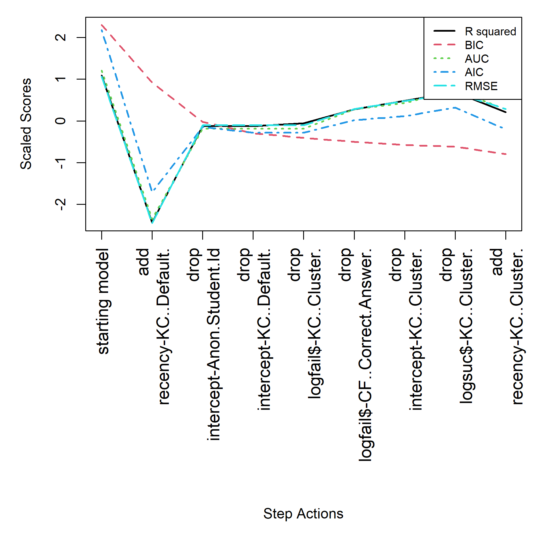
For the AFM start the final model is specified in feature(component) notation, see equation below. See Table 2 and Figure 1 for the step actions that led to this final model.

$$intercept(CF..Correct.Answer.) + recency(KC..Default.) + logsuc(CF..Correct.Answer.) + \ propdec(Anon.Student.Id)$$

For the BestLR start the final model is specified in feature(component) notation, see equation below. See Table 3 and Figure 2 for the step actions that led to this final model.

$$logsuc(Anon.Student.Id.) + logfail(Anon.Student.Id.) + intercept\ (CF..Correct.Answer.) + logsuc\$(CF..Correct.Answer.) + recency(KC.Default) + recency(CF..Correct.Answer.)$$

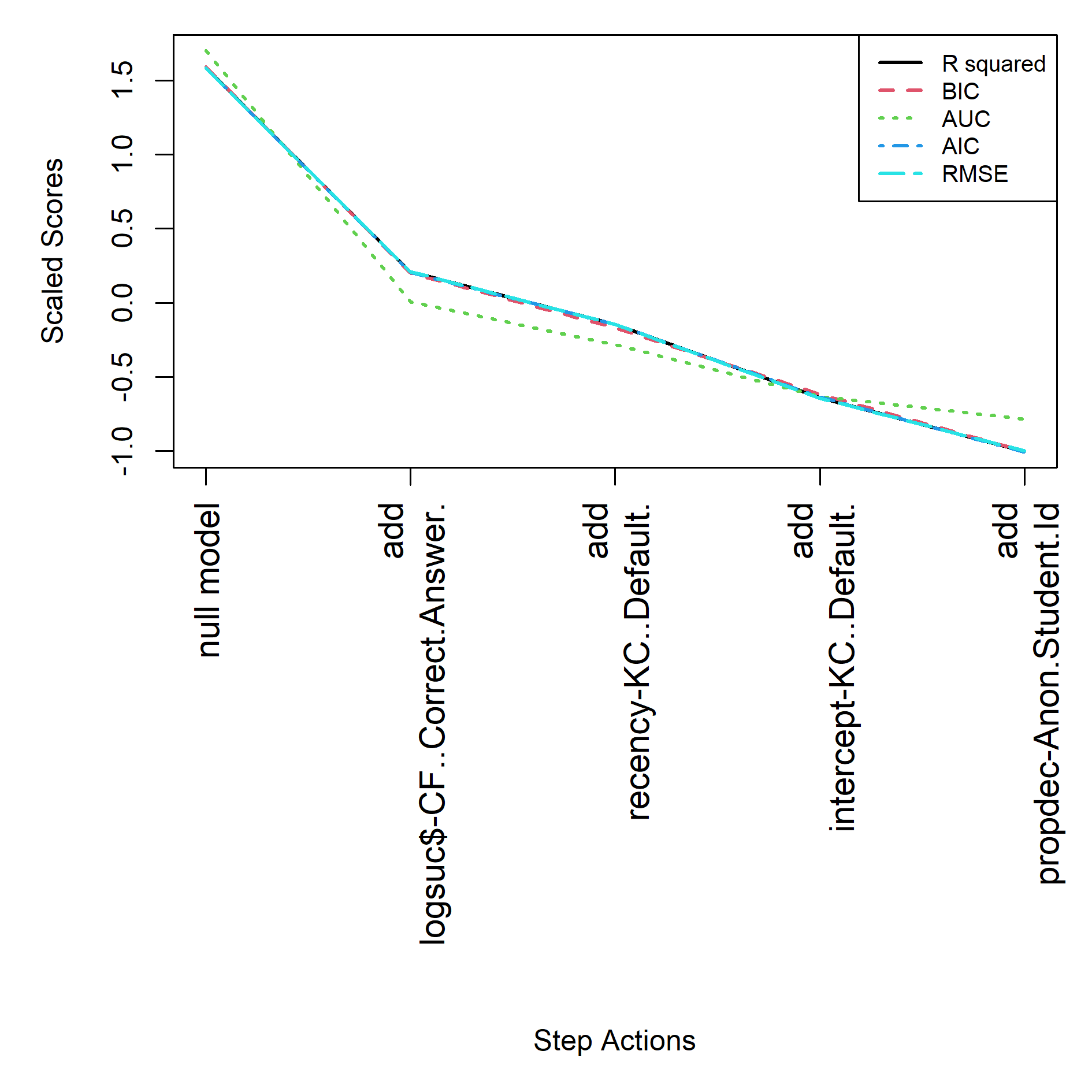
For the empty start the final model is specified in feature(component) notation, see equation below. See Table 4 and Figure 3 for the step actions that led to this final model.

$$logsuc\$(CF..Correct.Answer.) + recency(KC..Default.) + intercept(KC..Default.) + propdec(Anon.Student.Id)$$

MATHia Cognitive Tutor equation solving

The MATHia dataset included 119,379 transactions from 500 students from the unit Modeling Two-Step Expressions for the 2019-2020 school year. We used the student (Anon.Student.Id), MATHia assigned skills (KC..MATHia.), and Problem.Name as the item. This meant that our item parameter was distributed across the steps in the problems. There were 9 KCs and 99 problems. We chose not to use the unique steps as an item in our models for simplicity. This dataset included skills such as such as “write expression negative slope” and “enter given, reading numerals”.

Tables 5, 6 and 7 show the results for the different start models.

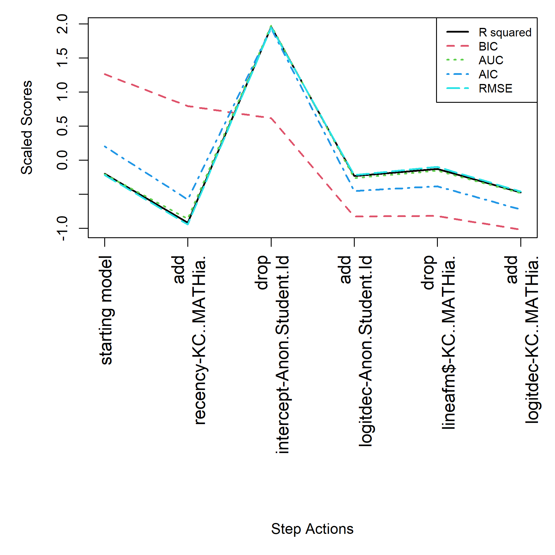
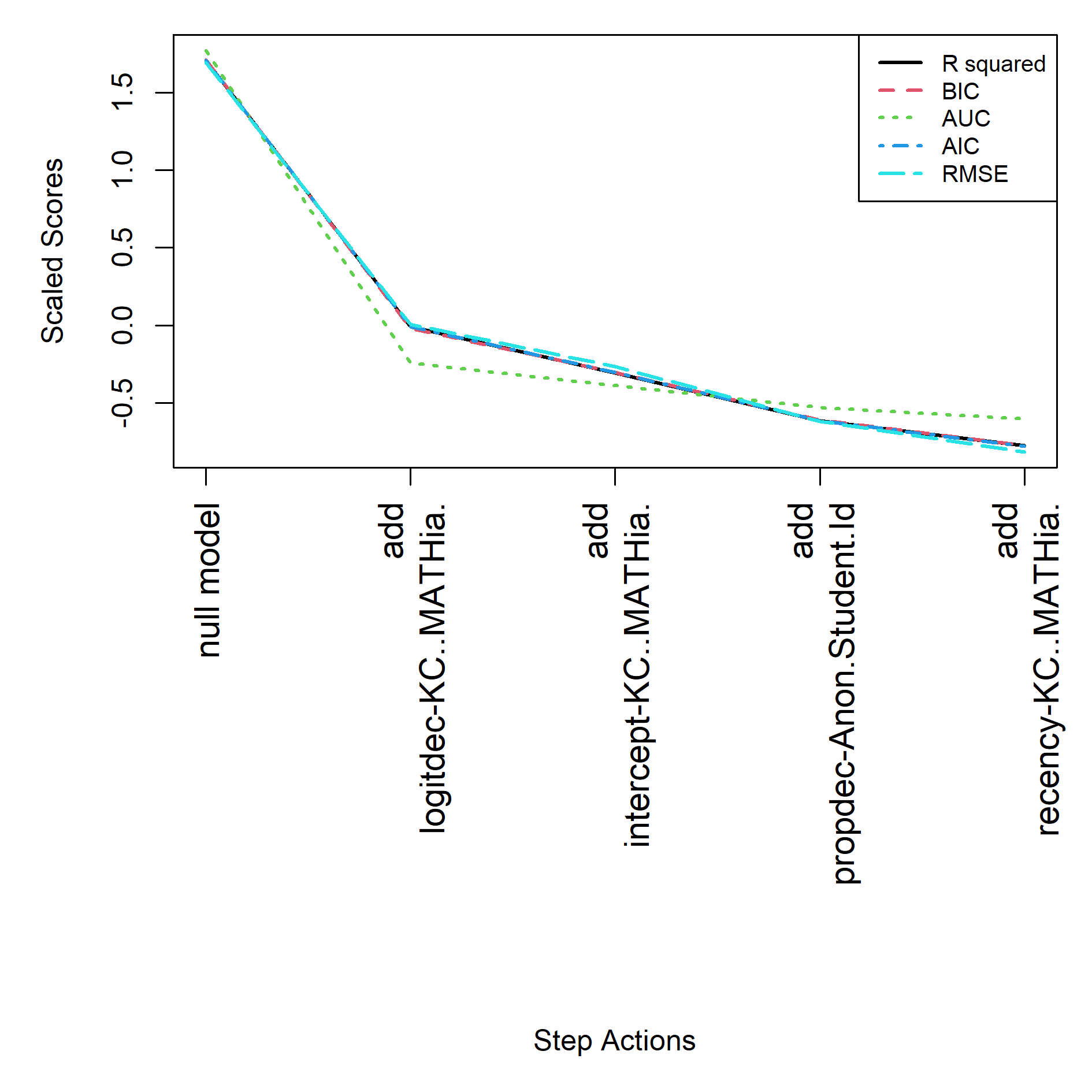
For the AFM start the final model is specified in feature(component) notation, see equation below. See Table 5 and Figure 4 for the step actions that led to this final model.

$$logitdec(Anon.Student.Id) + logitdec(KC..MATHia.) + recency(KC..MATHia.) + intercept(KC..MATHia.)$$

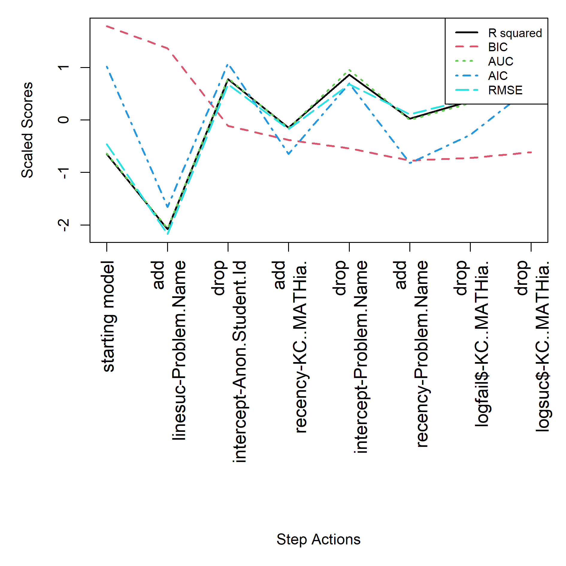
For the BestLR start the final model is specified in feature(component) notation, see equation below. See Table 6 and Figure 5 for the step actions that led to this final model.

$$logfail(Anon.Student.Id) + logsuc(Anon.Student.Id) + intercept(KC..MATHia.) + recency(KC..MATHia.) + recency(Problem.Name) + linesuc(Problem.Name)$$

For the empty start the final model is specified in feature(component) notation, see equation below. See Table 7 and Figure 6 for the step actions that led to this final model.

$$propdec(Anon.Student.Id) + intercept(KC..MATHia.) + recency(KC..MATHia.) + logitdec(KC..MATHia.)$$

Cloze with stepwise

For the cloze dataset, the models from the 3 starting points produce somewhat different results, illustrating the problem with any stepwise method due to it not being a global optimization. However, considering the fact that our goal is to practically implement these models, the result also suggests a solution to this local minima problem. By using more than one starting point we can identify the essential feature that explain the data.

For example, in these cloze results note that the recency feature used for the KC-Default is particularly predictive. In this dataset simply means that the time since the last verbatim repetition (KC Default) was a strong predictor with more recent time since last repetition leading to higher performance.

Successes were also important, but curiously they matter most for the KC-Correct-Answer. In all case the log of the success is the function best describing the effect of the correct responses. In this dataset, this mens that each time they responded with a fill-in word and it was correct, they would be predicted to do better the next time that word was the response. The log function is just a way to bias the effect of successes to be stronger for early succeses.

While the recency being assigned to the exact repetitions (KC-Default) indicates the importance of memory to performance, the tracking of success (as permanent effects) across like responses suggests that people are actually learning the vocabulary despite showing forgetting.

Consistent across all three final models is also the attention to student variability modeling. In BestLR, the log success and failure predictors for the student in the model mean that the student intercept is removed in an elimination step as redundant (this is also due to the BIC method, which penalizes the student intercept as unjustifiably complex). Interestingly, in the AFM and empty start models, we find that the propdec feature is added to capture the student variability after the intercept is removed, since there starts did not trace student performance with their start log success and failure feature as did BestLR from the start. The MATHia data has the same “problem” with BestLR start due to BestLR serving as enough of a local minima to block the addition of terms. More on this in the limitations section. Practically these features are important, since they allow the model to get an overall estimate for the student that greatly improves prediction of individual trials.

In summary, there appears to be no great advantage to starting with a complex starting model. Indeed, in all cases the stepwise procedure using BIC greatly simplifies the models by reducing the number of coefficients. It appears that prior models produced by humans (in this case, AFM and BestLR) do not produce better results in the model space than simply starting with an empty null hypothesis for the model. Furthermore, all three start models result in final models have no fixed student parameters, so should work for new similar populations without modifications, unlike AFM and BestLR which relied on fixed student intercepts

MATHia with stepwise

Practically speaking for the MATHia case we also see the importance of student variability, recency, and the correctness at fine grain by KC and item for all the models. Digging into the detail, ewe can see the BestLR start has some effect on the quantitative fit and chosen model. Most notably, while AFM and empty starts result in the student intercept being dropped in favor of logitdec and propdec respectively, the BestLR start retains the log success and failures predictors for the student. At the same time, Best LR, perhaps because it begins with the Problem.Name intercept as a covariate, adds features more features for Problem.Name, such as linesuc and recency. It seems clear that BestLR causes a different result. At this time, we might favor the simpler results of AFM or empty starts, but consider that the BestLR start fits the data by AUC slightly better than the BestLR result. This implies that AFM and empty starts are simply producing overly simplistic results. Consider we only dropped and removed terms when BIC gain was at least 500. We expect that running from an empty start to a lower BIC threshold would result in more commonality with BestLR start. To test this, we ran the empty start and indeed we found that the result became more similar to the BestLR result with the addition of linesuc and recency for the problems. Since this model (shown below) is still slightly worse than the BestLR start it implies that the algorithm favors composite features despite better fit from individual features (logsuc and logfail). We discuss this in the limitations and future work sections.

$$propdec(Anon.Student.Id) + intercept(KC..MATHia.) + recency(KC..MATHia.) + logitdec(KC..MATHia.) + linesuc\ (Problem.Name) + receny(Problem.Name)$$

Finally, all the models retained an intercept for the KCs, and all of the models capture MATHia KC performance change with the logitdec feature.

LASSO Method

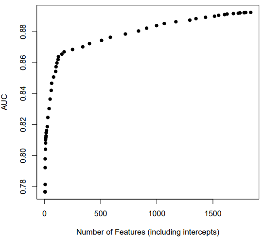
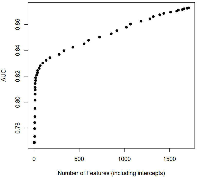
A primary goal of the LASSO analyses is to determine how well the approach can inform a researcher about which features are most important, and guide the researcher toward a fairly interpretable, less complex, but reasonably accurate model. See Figures 7 and 8 plotting the relationship between the number of features and AUC across 50 values of lambda ranging from .192 (a large penalty) to .0001 (very small penalty). For both datasets, there is clearly diminishing fit benefits as the number of features is increased (from a smaller lambda). Both curves have clear inflection points. At the inflection point, the coefficients for most features have been dropped to zero (see Table 8). Note in Table 8 that the MATHia dataset in particular fits quite well without many parameters for individual KCs. What remains appear to be the more robust and important features.

The final features that remained for LASSO models near the inflection points partially overlapped with those found with our stepwise regression approach as expected. Below the top 10 features for each dataset are listed in order of relative importance (see Tables 9, 10, and 11 below). When the results didn’t agree with the stepwise results, it appears that it may be because a stricter LASSO should be employed. For instance, a recency feature for the Problem.Name KC with decay parameter .1 remained in the MATHia dataset. However, it has a negative coefficient, which is challenging to interpret given that the negative sign implies correctness probability increases as time elapses. A larger lambda value may be justified.

For the Cloze dataset, a large number of features remained even at the inflection point (123) and they were missing many features we stepwise added. Inspecting the 123 features we saw that the variance stepwise captured in single terms was distributed across many terms in LASSO. Given that one goal of this work is to make simpler and more easily interpretable models for humans, we tried a larger penalty to reduce the number of features to 24. The resulting top 10 are in Table 10. This model is more interpretable to a human, with mostly recency features, recency-weighted proportion features, and counts of success for KC. While the match to stepwise is not exact we can now see it attending to student and KC successes and failures with features like logitdec in the top 10. It appears that lambda values are a sort a human interpretability index. Larger values make the resultant models more human interpretable, and in this case still create well-fitting models. Overall, the agreement between the approaches is encouraging evidence that these methods may be useful for researchers.

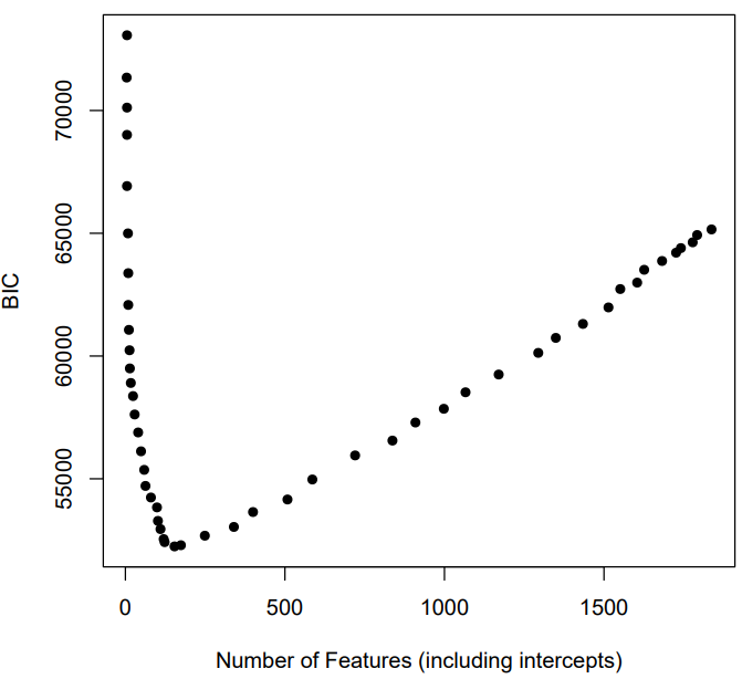
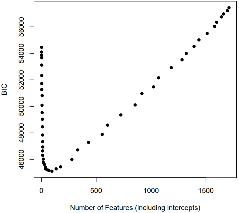
If minimum BIC is used instead of the AUC inflection point, the “optimal” models have slightly more features (e.g., 154 for cloze instead of 123, and 96 instead of 29 for MATHia), but still far fewer than the full model. The BIC minimum as a function of features is displayed in Figures 9 and 10.

Below in Table 12 we provide a final contrast of three example models with small, medium, and large lambda penalty terms. Interestingly, both datasets can achieve approximately AUC = .80 with ~10 features! Intercepts are considered features in this case, which means that a majority of the KC and student intercepts were dropped. This highlights a potential benefit of the LASSO approach for evaluating the fit of the KC model. It also suggested that student intercepts may not always be necessary in the presence of features like logitdec and propdec, which can stand in for intercepts to adjust for student differences.

Discussion

The results suggest both stepwise and LASSO methods work excellently to create, improve, and simplify student models using logistic regression. Both approaches generally agreed that recency features, logsuc, and recency-weighted proportion measures like propdec and logitdec were important. They also agreed that the number of necessary features was substantially less than the full models. While some have argued against stepwise methods [19], we think that stepwise methods worked relatively well here because the feature choices were not arbitrary. We did not simply feed in all the features we could find. Instead, we choose a set of features that can be theoretically justified.

Interpreting the results from these models needs to begin from consideration of the individual features. Each individual feature being found for a model means that the data is fit better if we assume the feature is part of the story for learning in the domain the data comes from. Clearly, we might expect different features for different domains of learning, and practically, knowing the features predicting learning means that we can better understand the learning better. For example, knowing that recency is a factor, or knowing that overall student variability is a big effect. The models this system builds might simply be used to understand online learning in some domain, but the expert building instruction technology might also use them in an adaptive learning environment to make decisions about student pedagogy or instruction.

Limitations and Future Work

A primary limitation of the present work is that we only included a subset of the features that are already known and established theoretically. There were also known features we did not include (e.g., specific time window features and interactions among features). An extension of this work will be to include more features as well as a step to generate and test novel features that may be counterintuitive. For instance, KC model improvement algorithms could be incorporated into the process [12]. However, how much variance is left to explain that is not covered by the set of features we used? With both datasets, models with AUC > .8 were found using only a relatively small subset of the potential features. Some fraction of unexplained variance is always to be expected due to inherent noise, KC model errors, and measurement error. A significant amount of remaining variance may be individual student differences that justify different types of models that update automatically to attempt to estimate individual learning rates, for example. These approaches are beyond the scope of this paper but an important topic for future work.

An opportunity for future work may also be to use these features as components in other model architectures, such as Elo or deep learning approaches. There are ongoing efforts to make deep learning models more interpretable, but for the present work we focused on a model architecture that is relatively interpretable to non-experts, logistic regression. Elo modeling is also particularly promising due to its simplicity and self-updating function [16]. Elo can be adjusted to include KT features like counts of successes and failures [11], but standard Elo without KT features also serves as a strong null model since it does reasonably well without KT features.

A key limitation of the stepwise method is the individuality of features. This is illustrated by the way that logsuc and logfail are retained in the BestLR MATHia model, but they are not added in any of the other models. Their retention in BestLR, may be best, but it may also reflect the standard tendency of stepwise methods to block the addition of new terms (possibly better) that are collinear with prior terms. This may be unavoidable, but also an uncommon problem we think. In contrast the fact that logsuc and logfail are not added for the student when nothing is already present might be because this requires 2 steps of the algorithm, while adding composite features like propdec or logitdec requires 1 step. Since stepwise selection is based on a greedy step optimization it ignores better gains that might occur in 2 steps.

A solution to this problem of feature grainsize, in which complex features are favored because they contain multiple sources of variability, might be to create synthetic linear feature groupings that can be chosen as an ensemble for addition to the model with each step. This was suggested by our results which showed logsuc and logfail being retained for the student for the BestLR start as discussed above. Future work will allow some “features” to actually test a combination of features for a component. Such a fix will allow us to add the combination feature logsuc and logfail (e.g., for the students) using 2 coefficients as usual, but in one stepwise step. This will allow it to compete with other terms such as logitdec or propdec, which incorporate success and failure already in the reported version here. More advanced methods can use factor selection which might be applied in both stepwise and LASSO within LKT, such as grouping specific features together such as KC models [21].

While the work here used BIC to reduce model complexity, and BIC works similarly to cross-validation in constraining unjustifiable complexity. We plan to confirm our results with out of sample validation methods in future work, also allowing us to further confirm that BIC is adequate. However, BIC likely underfits our final models relative to cross-validation [20]. So, it seems rather implausible that our models are invalid due to overfitting. Rather we may be running the risk of too little complexity, leaving explainable variability out of our model. Certainly, this highlights that out BIC stepwise threshold for addition and subtraction of terms was chosen arbitrarily to allow for interpretable models. We were pleased to see they also fit well.

Presets

To make the process of logistic regression modeling efficient, yet still retain some flexibility and user control, our tool includes a number of preset feature palettes that users will have available instead of specifying their own list. These presets are essentially a collection of theoretical hypotheses about the nature of the student model, given some goal of the modeler. The presets include the following four presets.

• Static - This present will contains only the intercept feature. It allows for neither dynamic nor adaptive solutions, essentially finding the best IRT type model, unless the item or KC component is not used, in which case it could simply find a single intercept for each student. Essentially it fits the LLTM model [5].
• AFM variants (i.e. dynamic but not adaptive) – This preset fits linear and log versions of the additive factors model[2], including LLTM terms that represent different learning rates or difficulties based on KC groupings (using the $ operator in LKT syntax).
• PFA and BestLR variants (dynamic and adaptive but recency insensitive) – This preset contains all of the above mechanisms, and also included the success and failure linear and log growth terms used in PFA [14] and BestLR[8].
• Simple adaptive – This catchall preset will include rPFA[7] inspired terms such as logitdec and propdec, described in the is paper and elsewhere [15]. In addition it will include temporal recency functions using only a single non-linear parameter, the best example of which, recency, was described in this paper and has been previously described [15].

Finally, future work might explore how Lasso also offers a convenient opportunity to evaluate the learner and KC model simultaneously. Within the Lasso approach, the coefficient of each KC can be pushed to zero and this could be used to allow refinement of the KC model. A limitation of our work here is that we did not explore this further, merely observing that in the models only some KCs were being assigned intercepts.

Conclusion

We find that the first few selected features in most models produced by the stepwise procedure are both effective AND interpretable. Articulating a theory to describe the simple models is relatively easy, since each feature can be justified by some research-based argument. For example, we see the importance of tracing student level individual differences in all the models, and we see the recency feature as indicating forgetting occurs. The LASSO procedure largely confirms the stepwise models are not far from a more globally optimal solution for our test cases and may reveal the future of the endeavor because of higher likelihood of a more global solution with LASSO despite the somewhat less interpretable models.

The present work sought to simplify the learner model building process by creating a model building tool, released as part of the LKT R package. Our promising interim results demonstrate too modes our tool has available to build models automatically. With stepwise, they can start with an empty model, provide sample data, and the fitting process will provide a reasonable model with a reduced set of features according to a preset criterion for fit statistic change. Alternatively, with the LASSO approach, the user provides data, and the resulting output will be a set of possible models of varying complexity based on a range of lambda penalties. The tool highlights models from lambda values based on minimum BIC and inflection points like those depicted in Figures 1 and 2.

ACKNOWLEDGMENTS

This work was partially supported by the National Science Foundation Learner Data Institute (NSF #1934745) project and a grant from the Institute of Education Sciences (ED #R305A190448).

REFERENCES

1. Cen, H., Koedinger, K., and Junker, B., 2006. Learning Factors Analysis: A General Method for Cognitive Model Evaluation and Improvement. In International Conference on Intelligent Tutoring Systems, M. Ikeda, K.D. Ashley and T.-W. Chan Eds. Springer, Jhongli, Taiwan, 164-176.
2. Cen, H., Koedinger, K.R., and Junker, B., 2008. Comparing two IRT models for conjunctive skills. In Proceedings of the Proceedings of the 9th International Conference on Intelligent Tutoring Systems (Montreal, Canada2008), 796-798.
3. Chi, M., Koedinger, K.R., Gordon, G., Jordan, P., and VanLehn, K., 2011. Instructional factors analysis: A cognitive model for multiple instructional interventions. In Proceedings of the 4th International Conference on Educational Data Mining (EDM 2011), M. Pechenizkiy, T. Calders, C. Conati, S. Ventura, C. Romero and J. Stamper Eds., Eindhoven, The Netherlands, 61-70. DOI= http://dx.doi.org/http://doi:10.1.1.230.9907.
4. Conati, C., Porayska-Pomsta, K., and Mavrikis, M., 2018. AI in Education needs interpretable machine learning: Lessons from Open Learner Modelling. arXiv preprint arXiv:1807.00154.
5. Fischer, G.H., 1973. The linear logistic test model as an instrument in educational research. Acta Psychologica 37, 6 (1973), 359-374. DOI= http://dx.doi.org/http://doi:10.1016/0001-6918(73)90003-6.
6. Friedman, J., Hastie, T., and Tibshirani, R., 2010. Regularization Paths for Generalized Linear Models via Coordinate Descent. J Stat Softw 33, 1, 1-22.
7. Galyardt, A. and Goldin, I., 2015. Move your lamp post: Recent data reflects learner knowledge better than older data. Journal of Educational Data Mining 7, 2 (2015), 83-108. DOI= http://dx.doi.org/https://doi.org/10.5281/zenodo.3554671.
8. Gervet, T., Koedinger, K., Schneider, J., and Mitchell, T., 2020. When is Deep Learning the Best Approach to Knowledge Tracing? JEDM| Journal of Educational Data Mining 12, 3 (2020), 31-54.
9. Gong, Y., Beck, J.E., and Heffernan, N.T., 2011. How to construct more accurate student models: Comparing and optimizing knowledge tracing and performance factor analysis. International Journal of Artificial Intelligence in Education 21, 1 (2011), 27-46. DOI= http://dx.doi.org/http://doi:10.3233/JAI-2011-016.
10. Khosravi, H., Shum, S.B., Chen, G., Conati, C., Tsai, Y.-S., Kay, J., Knight, S., Martinez-Maldonado, R., Sadiq, S., and Gašević, D., 2022. Explainable Artificial Intelligence in education. Computers and Education: Artificial Intelligence 3(2022/01/01/), 100074. DOI= http://dx.doi.org/https://doi.org/10.1016/j.caeai.2022.100074.
11. Papousek, J., Pelánek, R., and Stanislav, V., 2014. Adaptive practice of facts in domains with varied prior knowledge. In Proceedings of the 7th International Conference on Educational Data Mining (EDM 2014), J. Stamper, Z. Pardos, M. Mavrikis and B.M. Mclaren Eds., 6-13.
12. Pavlik Jr, P.I., Eglington, L., and Zhang, L., 2021. Automatic Domain Model Creation and Improvement. In Proceedings of The 14th International Conference on Educational Data Mining, C. Lynch, A. Merceron, M. Desmarais and R. Nkambou Eds., 672-676.
13. Pavlik Jr., P.I., Brawner, K.W., Olney, A., and Mitrovic, A., 2013. A Review of Learner Models Used in Intelligent Tutoring Systems In Design Recommendations for Adaptive Intelligent Tutoring Systems: Learner Modeling, R.A. Sottilare, A. Graesser, X. Hu and H.K. Holden Eds. Army Research Labs/ University of Memphis, 39-68.
14. Pavlik Jr., P.I., Cen, H., and Koedinger, K.R., 2009. Performance factors analysis -- A new alternative to knowledge tracing. In Proceedings of the 14th International Conference on Artificial Intelligence in Education, V. Dimitrova, R. Mizoguchi, B.D. Boulay and A. Graesser Eds., Brighton, England, 531–538. DOI= http://dx.doi.org/http://doi:10.3233/978-1-60750-028-5-531.
15. Pavlik, P.I., Eglington, L.G., and Harrell-Williams, L.M., 2021. Logistic Knowledge Tracing: A Constrained Framework for Learner Modeling. IEEE Transactions on Learning Technologies 14, 5, 624-639. DOI= http://dx.doi.org/10.1109/TLT.2021.3128569.
16. Pelánek, R., 2016. Applications of the Elo rating system in adaptive educational systems. Computers & Education 98(2016/07/01/), 169-179. DOI= http://dx.doi.org/https://doi.org/10.1016/j.compedu.2016.03.017.
17. Piech, C., Bassen, J., Huang, J., Ganguli, S., Sahami, M., Guibas, L.J., and Sohl-Dickstein, J., 2015. Deep Knowledge Tracing. In Proceedings of the Advances in Neural Information Processing Systems 28 (NIPS 2015) (2015), 1-9.
18. Schmucker, R., Wang, J., Hu, S., and Mitchell, T., 2022. Assessing the Performance of Online Students - New Data, New Approaches, Improved Accuracy. Journal of Educational Data Mining 14, 1 (06/24/2022), 1-45. DOI= http://dx.doi.org/10.5281/zenodo.6450190.
19. Smith, G., 2018. Step away from stepwise. Journal of Big Data 5, 1 (2018/09/15), 32. DOI= http://dx.doi.org/10.1186/s40537-018-0143-6.
20. Yates, L.A., Richards, S.A., and Brook, B.W., 2021. Parsimonious model selection using information theory: a modified selection rule. Ecology 102, 10 (2021/10/01), e03475. DOI= http://dx.doi.org/https://doi.org/10.1002/ecy.3475.
21. Yuan, M. and Lin, Y., 2006. Model selection and estimation in regression with grouped variables. Journal of the Royal Statistical Society: Series B (Statistical Methodology) 68, 1 (2006/02/01), 49-67. DOI= http://dx.doi.org/https://doi.org/10.1111/j.1467-9868.2005.00532.x.
22. Yudelson, M., Pavlik Jr., P.I., and Koedinger, K.R., 2011. User Modeling – A Notoriously Black Art. In User Modeling, Adaption and Personalization, J. Konstan, R. Conejo, J. Marzo and N. Oliver Eds. Springer Berlin / Heidelberg, 317-328. DOI= http://dx.doi.org/10.1007/978-3-642-22362-4_27.

© 2023 Copyright is held by the author(s). This work is distributed under the Creative Commons Attribution-NonCommercial-NoDerivatives 4.0 International (CC BY-NC-ND 4.0) license.